Otto cycle PV diagram program using Python

AIM: To plot an otto cycle PV diagram from initial and geometric parameters for an IC engine.

THEORY:

An Otto cycle canbe represented as Pressure vs Velocity graph of a IC engine combustion process. There are 4 set of stages for combustion in Otto cycle;

1. SUCTION STROKE: Here the inlet valves are open and air fuel ratio is let to flow in due to low pressure created by the piston when it moves from TDC to BDC.

2. COMPRESSION STROKE: This is also known as isentropic compression or a workinput stage where the valves are closed and air fuel mixture is trapped and compressed by the motion of piston from BDC to TDC.

3. Power/EXPANSION STROKE: This is know as a power stroke because the fuel is ignited here and a high pressure is generated and is known as heat addition and due to this the piston is pused from TDC to BDC.

4. EXHAUST STROKE: This is where the exhaust valves are open and burnt gases are pushed out by moving piston from BDC to TDC.

The Otto cycle consists of 4 process which will be used here to plot the graph which are;

1. Isentropic compression

2. Constant Volume heat addition

3. Isentropic expansion

4. Constant volume heat rejection

The Isentropic profile capturing is the major task here in this model which is captured using a formula as shown below;

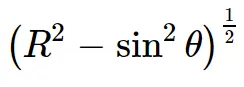
This equation will be used and splitted for better ease and solved here. The fuction is more useful here because there are multiple locations where we have repeat this process, so using a function is a better option.

METHOD:

The initial parameters and Geometric parameters are provided;

Intioal parameters-

P1 = 101325
T1 = 500
gamma = 1.4
T3 = 2500

Geometric parameters-

Bore = 0.1
Stroke = 0.1
Connecting_rod = 0.15
Compression_ratio = 8
Crank_pin_radius = Stroke/2
R = Connecting_rod/Crank_pin_radius

The program is attached below:-

import math
import matplotlib.pyplot as plt

def Volume_profile(Bore, Stroke, Connecting_rod, Compression_ratio, Start_angle, End_angle):

	Points = 50

	Swept_volume = math.pi*(1/4)*pow(Bore,2)*Stroke
	Clearance_volume = Swept_volume/(Compression_ratio - 1)

	sc = Start_angle
	ec = End_angle

	dtheta = (Start_angle - End_angle)/(Points - 1)
	V = []

	for i in range(0,Points):
		theta = sc + i*dtheta
		term1 = 0.5*(Compression_ratio - 1)
		term2 = R + 1 - math.cos(theta)
		term3 = pow(R,2) - pow(math.sin(theta),2)
		term3 = pow(term3,0.5)
		V.append((1 + term1*(term2 - term3))*Clearance_volume)
	

	return V




#Geometric Parameters
Bore = 0.1
Stroke = 0.1
Connecting_rod = 0.15
Compression_ratio = 8
Crank_pin_radius = Stroke/2
R = Connecting_rod/Crank_pin_radius


#Required inputs 
P1 = 101325
T1 = 500
gamma = 1.4
T3 = 2500

Swept_volume = math.pi*(1/4)*pow(Bore,2)*Stroke
Clearance_volume = Swept_volume/(Compression_ratio - 1)

V1 = Swept_volume + Clearance_volume

#start of constant volumme heat addition
V2 = Clearance_volume
P2  = P1*pow(V1,gamma)/pow(V2,gamma)
T2 = P2*V2*T1/(P1*V1)

V_compression = Volume_profile(Bore, Stroke, Connecting_rod, Compression_ratio, math.pi, 0)
P_compression = []

for v in V_compression:
	P_compression.append(P1*pow(V1,gamma)/pow(v,gamma))


#Start of isentropic expansion
V3 = Clearance_volume
P3 = (P2*V2/T2)*(T3/V2)

#Start of Constant Volume heat rejection
V4 = V1
P4 = P3*pow(V3,gamma)/pow(V4,gamma)
T4 = P4*V4*T3/(P3*V3)



V_expansion = Volume_profile(Bore, Stroke, Connecting_rod, Compression_ratio, 0, math.pi)
P_expansion = []

for v in V_expansion:
	P_expansion.append(P3*pow(V3,gamma)/pow(v,gamma))

#Thermal efficiency

Therm_eff = (1 - (T4-T1)/(T3-T2))*100
print('Therm_eff =', Therm_eff)


plt.plot([V2,V3],[P2,P3])
plt.plot(V_compression,P_compression)
plt.plot([V1,V4],[P1,P4])
plt.plot(V_expansion,P_expansion)
plt.xlabel('Volume')
plt.ylabel('Pressre')
plt.show()

The program ran and the results are below attached.

RESULTS:

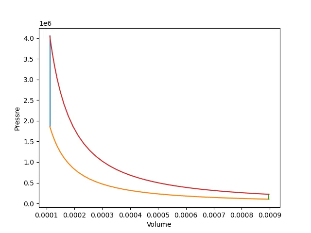
PV diagram for compression ratio 8:-

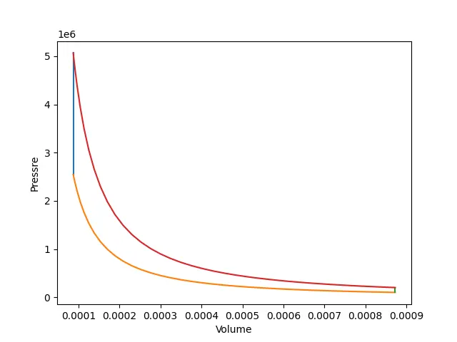
PV for compression ratio 10:-

PV diagram for cr_12:-

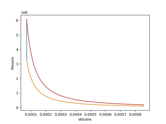
We can see that as the compression ratio increases the P2 value increases and similarly efficiency also increases.

Thermal efficiency for cr_8 = 56.4724

Thermal efficiency for cr_10 = 60.1892

Thermal efficiency for cr_12 = 62.9892

CONCLUSION:

The case was ran successfully with different compression ratios and absorved the variation in thermal efficiency.