One Dimensional Linear Convection - Effect of Time Step on Solution

Write a function that accepts the time step as an argument and solves the same problem. You will compare the effect of the time step on the numerical solution.

1. Number of nodes, n = 80

2. Time step , dt = 1e-4, 1e-3, 1e-2, and 1e-1

3. Simulation run time , t = 0.4 seconds.

Solution:

Given,

Grid size n = 80

Time Steps = 1e-4, 1e-3, 1e-2 and 1e-1

Simulation time = 0.4 seconds

1D linear convection equatioin

`(u^(n+1)-u^n)/(Deltat)+C((u_i-u_(i-1))/(Deltax))=0`

MATALAB Coding

%Effect of time step size on the solution
clear all
close all
clc

L=1;
n=80;
c=1;
t_end=0.4;
dt=[1e-4 1e-3 1e-2 1e-1];

%calculations
x=linspace(0,L,n); %size of domain
dx=L/(n-1); %grid size

%defining the nodes at velocity 2m/s
x_start=0.1;
x_end=0.3;

%time marching solutions
nt1=t_end/dt(1);
nt2=t_end/dt(2);
nt3=t_end/dt(3);
nt4=t_end/dt(4);

%evaluating nodes at start and end 
n_start=0.1/dx+1;  
n_end=0.3/dx+1;   

%initialling arrays & applying boundary condition
u=ones(1,n);
u(n_start:n_end)=2;

%boundary conditions u(1)=1
u_old=u;
u_initial=u;

%execution time interval
t_exe=zeros(1,4);

tic

% time loop (1e-4)
for k=1:nt1
    
    %space loop
    for i=2:n
         u(i)=u_old(i)-(c*dt(1)/dx)*(u_old(i)-u_old(i-1));
    end
    
    %updating old velocities
    u_old=u;
    t_exe(1)=toc;
end

%initialling arrays & applying boundary conditions
u1=ones(1,n);
u1(n_start:n_end)=2;

%boundary conditions u(1)=1
u1_old=u1;
u1_initial=u1;

tic

% time loop (1e-3)
for k=1:nt2
    
    %space loop
    for i=2:n
         u1(i)=u1_old(i)-(c*dt(2)/dx)*(u1_old(i)-u1_old(i-1));
    end
    
    %updating old velocities
    u_old=u1;
    t_exe(2)=toc;
end

%initialling arrays & applying boundary conditions
u2=ones(1,n);
u2(n_start:n_end)=2;

%boundary conditions u(1)=1
u2_old=u2;
u2_initial=u2;

tic

% time loop (1e-2)
for k=1:nt3
    
    %space loop
    for i=2:n
         u2(i)=u2_old(i)-(c*dt(3)/dx)*(u2_old(i)-u2_old(i-1));
    end
    
    %updating old velocities
    u2_old=u2;
    t_exe(3)=toc;
end

%initialling arrays & applying boundary conditions
u3=ones(1,n);
u3(n_start:n_end)=2;

%boundary conditions u(1)=1
u3_old=u3;
u3_initial=u3;

tic

% time loop (1e-1)
for k=1:nt4
    
    %space loop
    for i=2:n
         u3(i)=u3_old(i)-(c*dt(4)/dx)*(u3_old(i)-u3_old(i-1));
    end
    
    %updating old velocities
    u3_old=u3;
    t_exe(4)=toc;
end


%plottings
figure(1)
plot(x,u,x,u1,x,u2,x,u3,'linewidth',2);
grid on
axis([0 1 0 2.5])
xlabel('Length of Domain')
ylabel('velocity')
legend('1e-4','1e-3','1e-2','1e-1')
title('comparsion of the velocity profiles for various time steps at T=0.4')

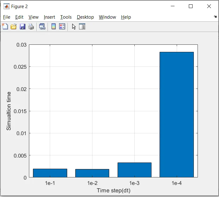
figure(2)
y=categorical({'1e-4','1e-3','1e-2','1e-1'});
bar(y,t_exe)
grid on
xlabel('Time step(dt)')
ylabel('Simualtion time')

Output:

Comparison of the effect of Time Step on the Numerical Solution

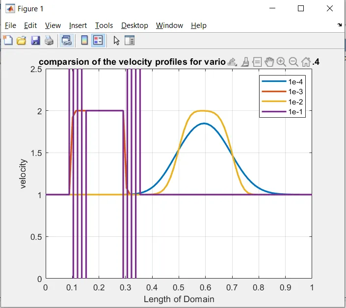
From the above plot, we can see that for the first time step, the solution is blowing out implying that the solution is unstable. it can be explained with respect to the method used i.e. an explicit method is susceptible to the time step given, which results in an unstable solution. so the time step has to be correct or within the viable range for the solution. This can be determined by a condition called Courant-Friedrichs-Lewy (CFL) condition. It is a necessary condition for convergence while solving certain PDEs numerically.

1D equation of linear convergence the CFL has the following form:

`C = (uDeltat)/(Deltax)le C_max`

where C is Courant Number which is dimensionless