One Dimensional Linear Convection

Numerical solution to the One-dimensional Linear Convection equation.

1. Assume that the domain length is L = 1m

2. The initial velocity profile is a step function. It is equal to 2m/s between x= 0.1 and 0.3 and 1m/s everywhere else

3. Use first-order forward differencing for the time derivative

4. Use first-order backward/rearward differencing for the space term.

5. Constant convection coefficient, c = 1 m/s

6. Time step, dt = 0.01

7. Simulation run time , t = 0.4 seconds.

Perform the simulation for Number of nodes, n=20,40,80 and 160.

Solution:

General equation for linear convection:

`(delu)/(delt)+C(delu)/(delx)=0`

where,

Set time step = 0.01

Constant velocity C = 1m/s

Making comparison for n = 20, 40, 80 and 160

By applying forward difference scheme for time and backward difference scheme for space we get:

`(u^(n+1)-u^n)/(Deltat)+C((u_i-u_(i-1))/(Deltax))=0`

MATLAB Coding

% One_dimentional_linear_convection
clear all
close all
clc
% ginven inputs
L = 1;
n = [20 40 80 160];
c = 1;
t = 0.4;
dt = 0.01;

% nodes at velocity 2m/s
x_start=0.1;
x_end=0.3;

% time marching solution
nt=t/dt;

%obtain velocity profiles for all values of n
for i=1:length(n)
    
    %calculations
    %domain size
    x=linspace(0,L,n(i));
    % grid size
    dx=L/(n(i)-1); 
    
    
    %creating array at nodes for velocity is 1m/s
    u=ones(1,n(i));
    
    %evaluating nodes at start and end for various values of i
    n_start(i)=round((x_start/dx)+1);
    n_end(i)=round((x_end/dx)+1);
    
    %defining nodes at velocity is 2m/sec
    u(n_start(i):n_end(i))=2;
    
    %boundary conditions
    uold=u;
    u_initial=u;
    
    %time marching solution
    
    % time loop du/dt
    for j=1:nt
         
        %space loop 
         for k=2:n(i)
             %backward differencing
            u(k)=uold(k)-(c*dt/dx)*(uold(k)-uold(k-1)); 
         end
        
        %update old velocity
        uold=u;
        
        %plotting 
        figure (1)
        plot(x,u_initial,'r','linewidth',2)
        hold on
        grid on
        plot(x,u,'b')
        axis([0 1 0 2.5])
        hold off
        xlabel('length of domain')
        ylabel('velocity')
        legend("Initial velocity","Velocity at time step")  
        
    end
        
end

Output:

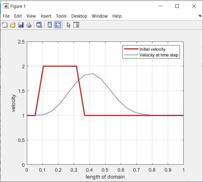
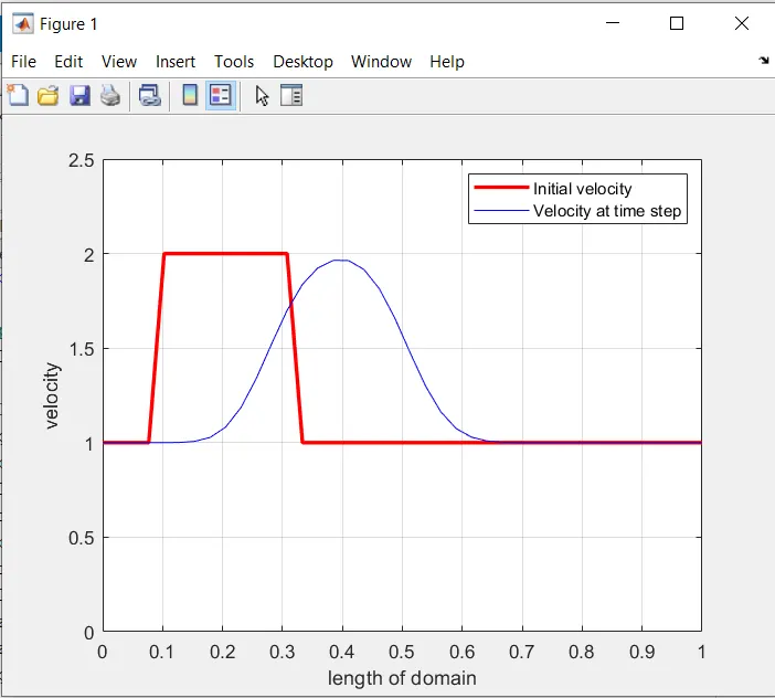
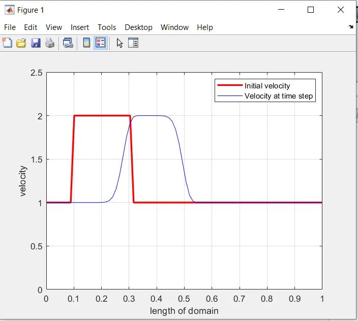
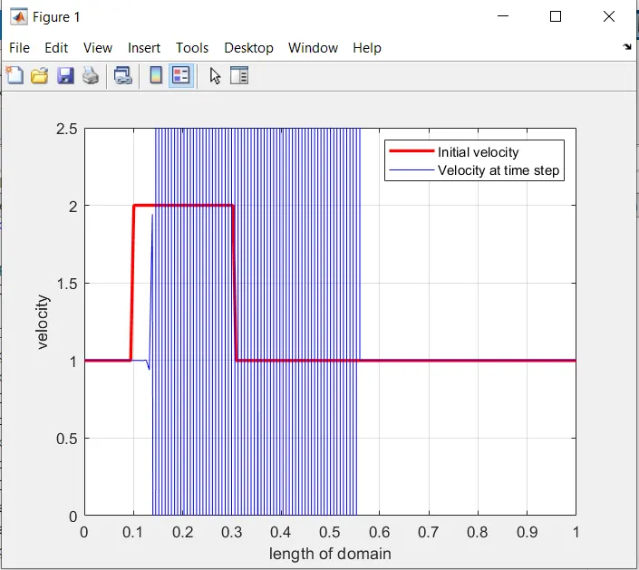
Comparision of original velocity and final velocity profiles

for n=20

for n=40

for=80

for=160

Conclusion:

By observing the about polts, one can say that the accuracy of the solution increases as the number of grid points increases however, at a certain threshold value of n the result is in-accurate and hence it is important to select the correct grid size.