Abstract:

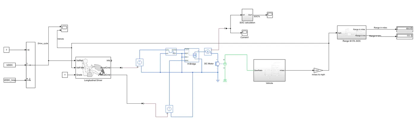
This project describes the physical modelling and simulation of a battery-powered Electric Vehicle controlled by H-bridge and PWM voltage controller. The UDDC drive cycle is used to run the model. The model is simulated until 5% SOC of the battery and the range is estimated. The speed of vehicle approximately follows the drive cycle.

Introduction:

The model is created in Simulink environment by using Simscape toolset. This toolset is used for physical modelling of the system. It behaves as a physical system and replicates approximately the real scenario by considering all the errors, inertia, damping etc. which is very difficult to model through Simulink blocks by using equations. The voltage supplied to motor is controlled by H-bridge and PWM controller. These configurations have reduced the complexity of the overall model by making it simple but effective. There are some Simulink blocks used in the model which are connected to physical blocks with the help of ‘Physical system to Simulink convertor’. This is because the physical blocks signals cannot be directly connected to Simulink blocks and vice versa.

Electric vehicle parameters:

The parameters used are taken from BMW i3 model:

Parameters	Values
Mass (Considering passenger)	1772 kg
Max. Power	165 kw
Max. Torque	250 Nm
Rated Power	75 kw
Rated rpm	4800 rpm
Battery capacity	120 AH
Battery voltage	352 V
Gear Ratio	9.665

Vehicle dynamics:

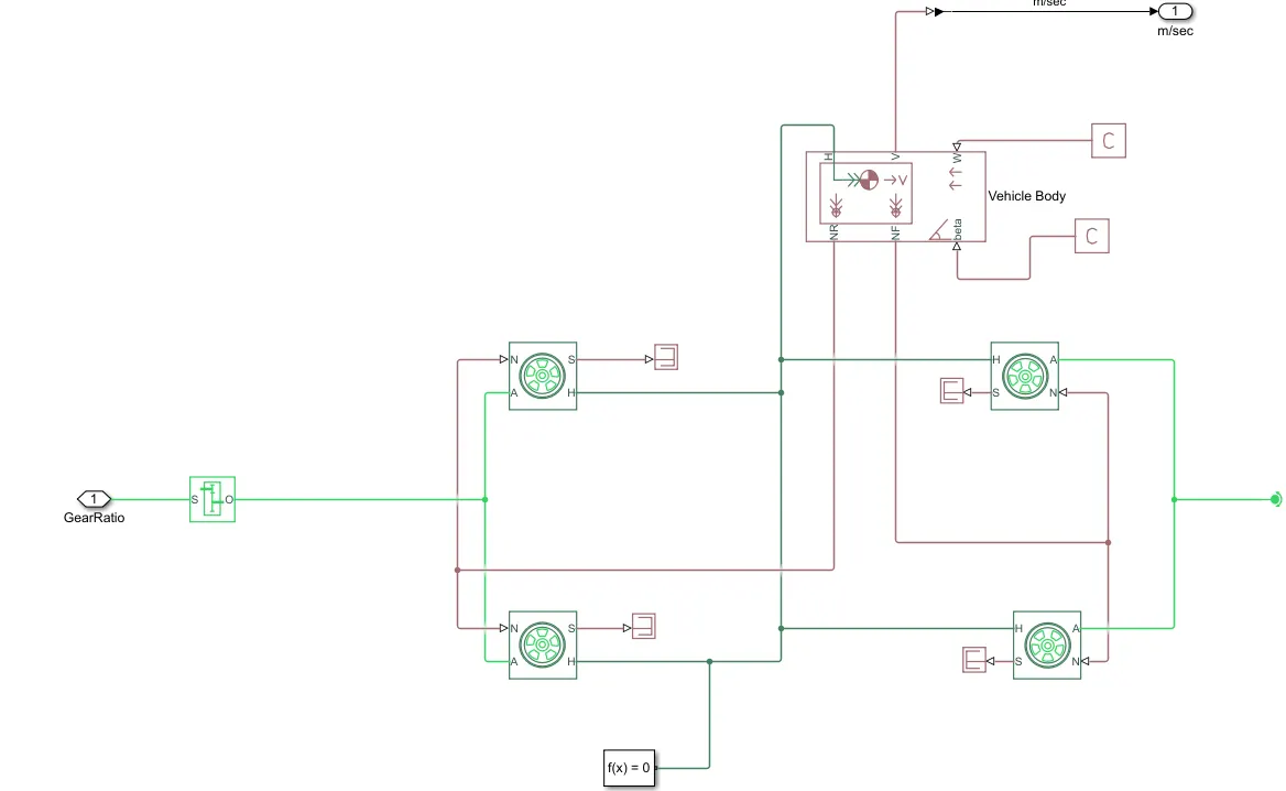
The vehicle dyanamic is concerned with the movement of vehicle on the road surface. The Dynamic behaviour of the vehicle is determined by the forces imposed on vehicle from road wheels, gravity and aerodynamic drag force.

The vehicle dynamics works on Newton’s 2nd law which states that when a body is in motion, the forces acting on it is equal to it’s mass multiplied by acceleration.

m*a = Ft

In case of vehicle the net tractive force have to overcome a couple of resistive forces such as aerodynamic drag force, rolling reistance force and hill climbing or grade force.

m*a = F_t – F_resist

Aerodynamic drag force depends on two components i.e shape drag and skin friction. It is the function of frontal area, shape and air passage etc of the vehicle.

F_a = ½*rho*af *C_d*v^2

Where ‘af’ is the vehicle’s frontal area, ‘C_d’ is the drag coefficient, ‘rho’ is the density of air and ‘v’ is the velocity at which the vehicle is moving.

Rolling resistance is caused by hysteresis present in wheel loading and unloading, and creates a moment that opposes the rotation of the wheel. However, rolling resistance is simplified and represented as an equivalent force acting at the wheel's center, given by the equation:

Frr = m*g*fr*cos

where ‘m’ is the mass, ‘g’ is the gravitational force, ‘fr’ is the rolling resistance coefficient, is the road inclination angle

Grade resistance is the component of the vehicle's weight acting parallel to the road surface, and is given by:

Fg = m*g*sin

The tractive force Ft is calculated from the torque generated from the motor :

Ft = T*g_r/r_w

where ‘T’ is the torque, ‘g_r’ is the gear ratio, ‘r_w’ is the radius of wheel

The resistive force is given by :

F_resist = Fa + Frr + Fg

Hence acceleration is calculated by:

a = (F_t – Fa – Frr – Fg) / m

Further the velocity is calculated by integrating the acceleration which is the output of vehicle dynamic.

This all above equations is taken care by the physical block ‘Vehicle’ and ‘Tyre’. The vehicle is connected by the 4 wheels. The power from motor is supplied to the rear wheels hence it is a rear wheel drive.

Gear box is used with a gear ratio of ‘9.665’.

DC motor:

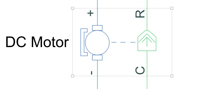
This physical block represents the electrical and torque characteristics of a DC motor.The block assumes that no electromagnetic energy is lost, and hence the back-emf and torque constants have the same numerical value when in SI units. Motor parameters can either be specified directly, or derived from no-load speed and stall torque. If no information is available on armature inductance, this parameter can be set to some small non-zero value.

H-Bridge:

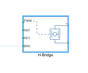
This block represents an H-bridge motor drive. The block can be driven by the Controlled PWM Voltage block in PWM or Averaged mode. In PWM mode, the motor is powered if the PWM port voltage is above the Enable threshold voltage. In Averaged mode, the PWM port voltage divided by the PWM signal amplitude parameter defines the ratio of the on-time to the PWM period. Using this ratio and assumptions about the load, the block applies an average voltage to the load that achieves the correct average load current. The Simulation mode parameter value must be the same for the Controlled PWM Voltage and H-Bridge blocks.

If the REV port voltage is greater than the Reverse threshold voltage, then the output voltage polarity is reversed. If the BRK port voltage is greater than the Braking threshold voltage, then the output terminals are short circuited via one bridge arm in series with the parallel combination of a second bridge arm and a freewheeling diode. Voltages at ports PWM, REV and BRK are defined relative to the REF port.

Controlled PWM Voltage:

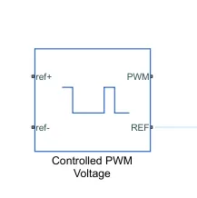
This block creates a Pulse-Width Modulated (PWM) voltage across the PWM and REF ports. The output voltage is zero when the pulse is low, and is equal to the Output voltage amplitude parameter when high. Duty cycle is set by the input value.

At time zero, the pulse is initialized as high unless the duty cycle is set to zero or the Pulse delay time is greater than zero.

Driver Controller:

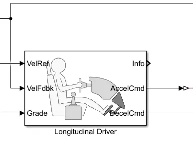
A parametric longitudinal speed tracking controller for generating normalized acceleration and braking commands based on reference and feedback velocities.

The velocity from the driving cycle is substracted from the velocity of the vehicle dynamics and the error is obtained which is to be control so that the input and output velocity should exactly match.

The error is sent as an input to PI controller where the tuning is done.

The acceleration and braking commands are generated which is fed to 'Controlled PWM Voltage' and 'H-Bridge'.

Drive Cycle:

A driving cycle is a series of data points representing the speed of a vehicle versus time. Driving cycles are produced by different countries and organizations to assess the performance of vehicles in various ways, as for example fuel consumption and polluting emissions.

In this case the Urban Dynamometer Driving Schedule (UDDS) cycle is used and it will run in the loop till the State of Charge(SOC) of the battery is 5 percent. The output of the driving cycle is the velocity with respective time.

SOC calculation:

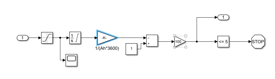
In this model, the current calculated from the motor model is actually the current demanded by the motor from the battery to run which is assumed that it is given by the battery.

This current is used to calculate State Of Charge (SOC) of the battery. To calculate the SOC, this current is first integrated which gives current in Ampere second and then this current is divided by 3600 to get current in Ampere hour. The calculated Ampere hour(Ah) is divided by actual current capacity of the battery which is 120Ah, then the output is substracted from 1 and multiplied by 100 to get the SOC in percentage.The simulation should stop when the battery SOC is about 5 percent. For this purpose ‘Stop Simulation’ block is used.

Results:

1. Targeted Vs Simulated Voltage in mph:

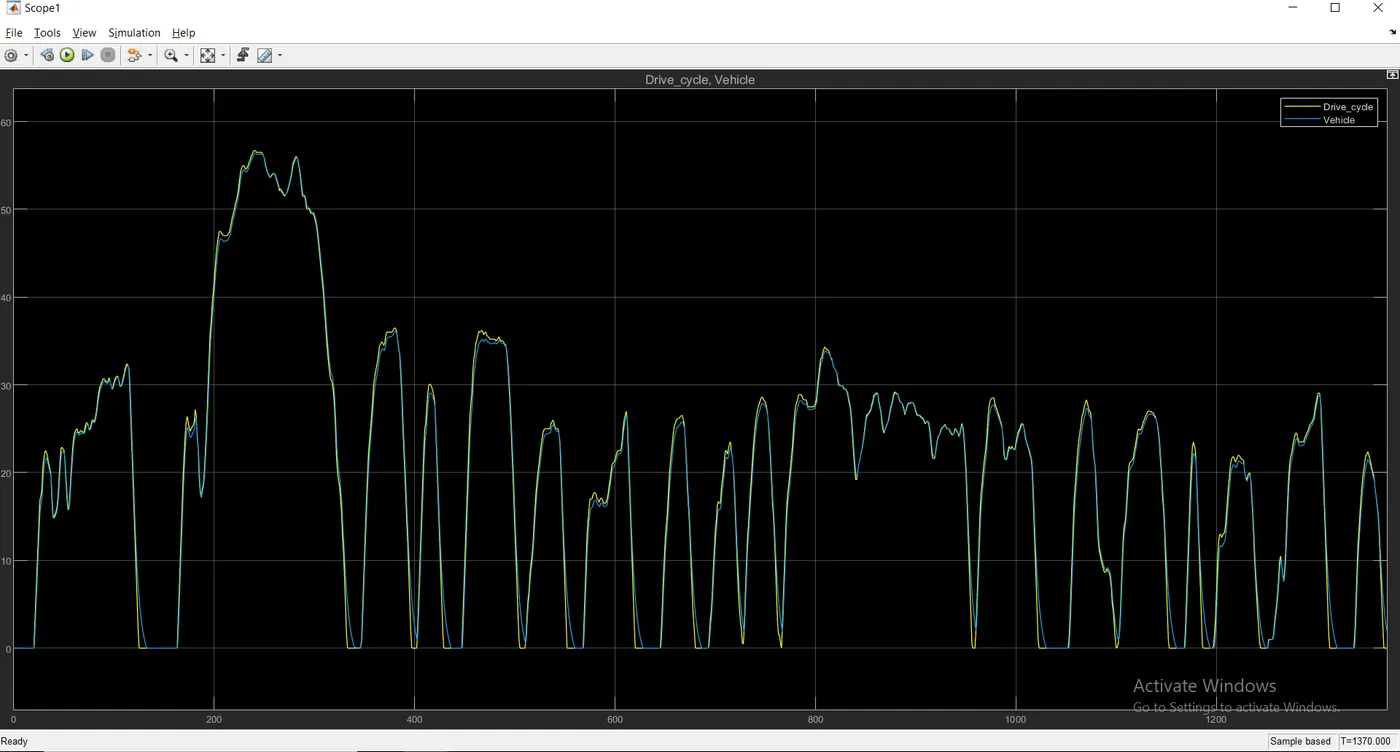
As seen in the above graph that the velocity from the vehicle approximately matches to the target velocity of the drive cycle, hence we can say that our vehicle is following the drive cycle and the desired behavior is obtained.

2. SOC for single UDDC cycle:

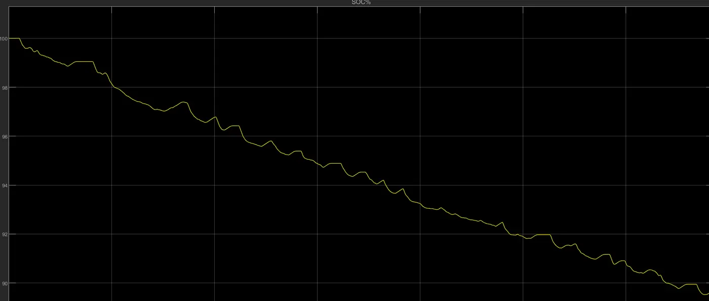
The above graph shows the SOC of the battery. Here we can see that for a single UDDC cycle the SOC is 89% i.e 89% of charge is left inside the battery when vehicle is run for single UDDC cycle for 1370 seconds. The humps in the graph indicate that the battery is being charged due to regeneration braking.

3. Range untill 5% SOC:

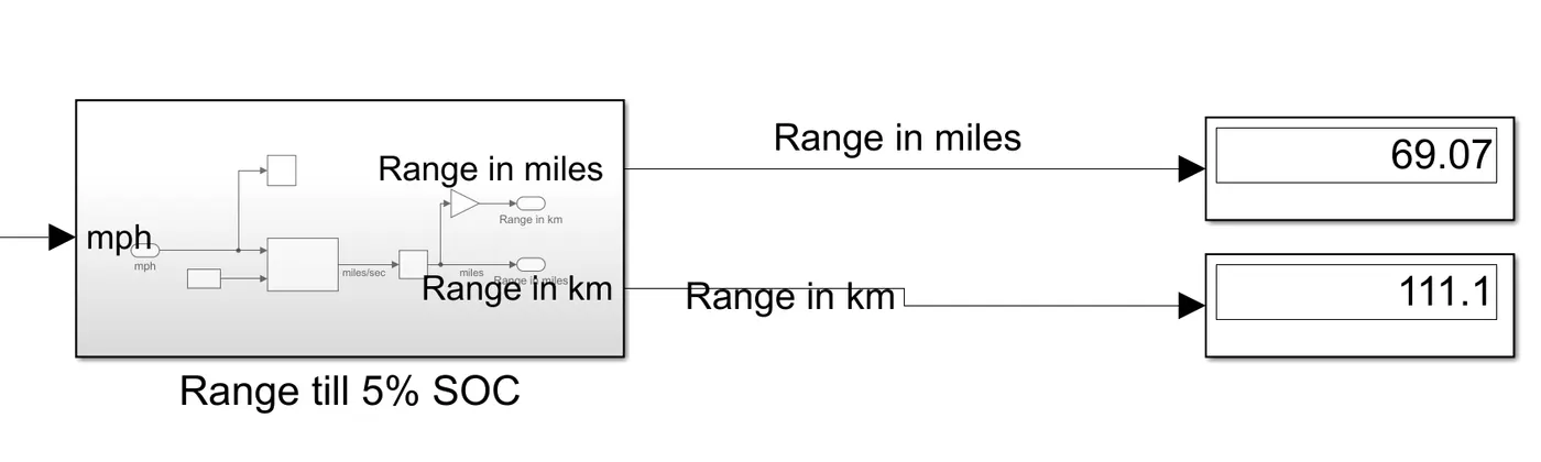
The UDDC drive cycle is run in a loop until we get 5% SOC. For 5% SOC the range is 69.07 miles and 111.1 km.

4. Current supplied to Motor:

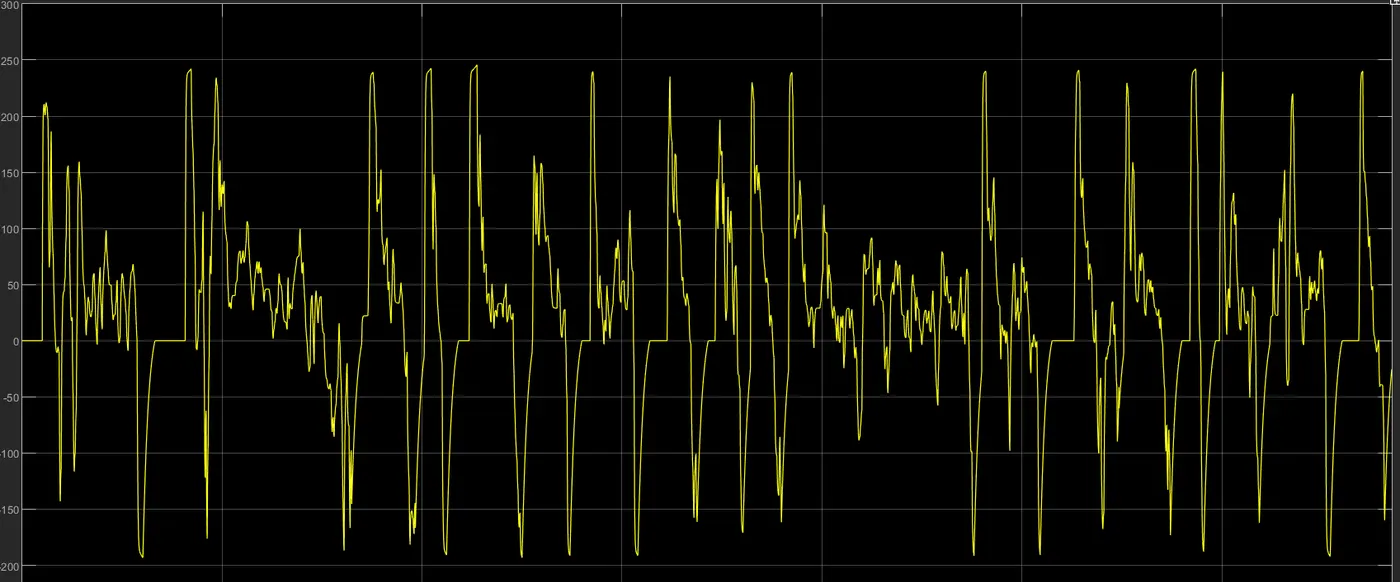
The above graph shows the current supplied to the DC motor. The positive current indicates that the energy is being utilized by the vehicle and battery is discharged. The negative current indicates that the charge is being supplied to the battery due to regeneration braking.

Conclusion:

Hence the subsystem of typical electric vehicle is modelled by using the physical toolset and the desired results have been obtained. The advantage of a concise and transparent toolset lies in its ease of adaptability to almost any scenario, and its low learning overhead allows students and professionals alike to modify even its core components to fit an application. Tools like this can be used to quickly and cheaply validate vehicle designs, including “think-outside-the-box” or radical designs.

First-pass component sizing and system-level optimization studies can also be performed without the need for expensive laboratory experiments. The forward-looking nature of this toolset also allows future users to perform control system optimization studies as well as hardware-in-the-loop (HIL) Simulation.