Modeling and Simulation of flow around an Ahmed Body
Introduction
The objective of the current study is to simulate air flow over an Ahmed Body with a slant angle of 35º. Simulations are carried out on a standard Ahmed Body for a fixed inlet velocity and the resulting drag and lift coefficients are plotted and studied.
Designed by S.R. Ahmed, an Ahmed Body is somehwat of a benchmark for simulations in the automotive and aerodynamic fields. Its unique geometry enables the user to accurately simulate the major phenomena that take place when a fluid flows over a conventional automobile, namely a large displacement flow in the front, uniform flow through the central portion, and a considerable wake in the rear segment of the body. Its primary advantage is its relative ease to model, while simultaneously producing accurate results.
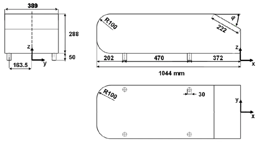
Two of the primary aerodynamic forces acting on an Ahmed Body are the Drag and Lift forces. Unlike an airfoil, automobiles are designed to generated a negative lift, also known as the downforce, to ensure the vehicle stays in contact with the ground. These two forces are calculated as shown below:
`D=1/2*rho*A*v^2*Cd`_______________i
`L=1/2*rho*A*v^2*Cl`_______________ii
where `D` is the Drag Force, `L` is the Lift force, `rho` is the density of the fluid, `A` is the acting area of the fluid, `v` is the free stream velocity of the fluid, `Cd` and `Cl` refer to the drag and lift coefficients respectively.
Computational Details and Case Setup
The Ahmed body geometry is designed in Catia V5, as shown in below. An additional body, in the shape of a rectangle is constructed. The Ahmed Body is subtracted from the rectangular body to obtain the wind tunnel needed for the case setup. The dimensions of the wind tunnel are calculated as follows:
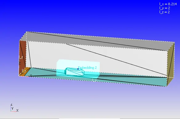
The problem statement specifies a boundary layer thickness of 30 mm at a distance of 400 mm from the Ahmed body. The boundary layer thickess `delta`is given as
`delta=(0.382*x)/((Rex)^(1/3))`_______________iii
where `x` is the length of the plate and `Rex` is the Reynolds number at `x`
`Rex` is given as
`Rex=(v*x)/nu`_______________iv
where `v=40` m/s and `nu` is the kinematic viscosity of air and is equal to `1.552*10^(-5)` (m^(2)/s)
Substitute iv in iii to get the value of x as ~1.67 m.
Since the problem statement specifies the thickness of the boundary layer as 30 mm at a distance of 400 mm before the Ahmed body in addition to a free slip region of 300 mm, the length of the wind tunnel on the upstream side of the Ahmed body is calculated as
`Lup=0.3+1.67+0.4=2.37m`
To accurately capture the fluid dynamics in the wake region, the length of the downstream portion of the `Ldown` is taken as 4.8 m.
Therefore, length of the wind tunnel is given as `Lw`in`d=2.37+1.044+4.8=8.214 m`
The width and height of the wind tunnel are taken as 2 m each.
Following this, the geometry is imported as an STL file into Converge Studio. The boundary conditions utilised in this simulation are shown below
| Boundary Name | Condition |
| Inlet | Inflow: Axial velocity= 40 m/s, Pressure: 150000 Pa |
| Outlet | Outflow: Velocity: NE BC, Pressure= 101325 Pa |
| Free slip region | Wall: Slip condition, TKE: NE, Omega: NE |
| Ahmed Body | Wall: Law of Wall, TKE: NE, Omega: Wall Model |
| No Slip | Wall: Law of Wall, TKE: Ne, Omega: Wall Model |
| Symmetry (Top and lateral surfaces) | Symmetry BC |
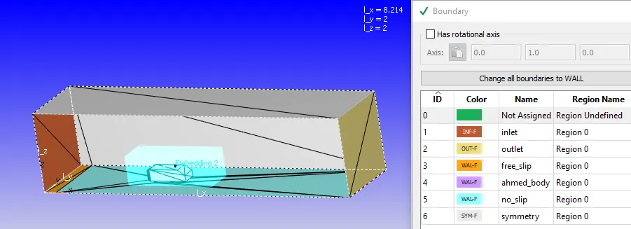
It is crucial to carry out a dianosis check of the imported geometry into Converge Studio to check for intersecting and non-manifold edges/triangles.
A fully hydrodynamic, compressible, transient solver operating on the PISO algorithm is chosen for the current simulation. The total simulation time is determined to be ~4 times the mean flow time of the fluid, which is calculated as Lwind/`v`, which is equal to `4*8.214/40=0.82 s`
The `k-omega SST` turbulence model has been adopted for the current study. Since the drag and lift forces are primarily studied in the viscous sublayer and buffer region, it is logical to opt for a turbulence model that accurately predicts wall behaviours for low values of Y+. The entire region was initialised with an axial velocity of 40 m/s and a temperature of 300 K.
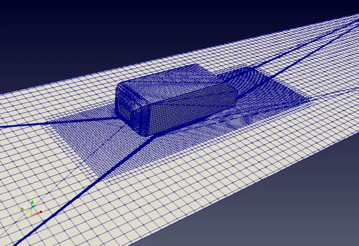
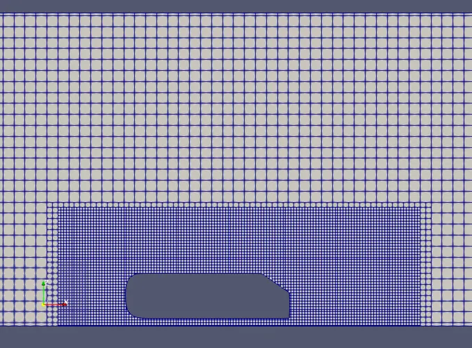
A structured mesh with a base grid of 0.7 m is initially adopted due to computational restrictions. However, to improve the accuracy of the obtained results, a layer of fixed embedding is applied on a cuboidal area around the Ahmed body. The scale of fixed embedding was fixed at 2 for the duration of the simulation and is shown below.
Results and Discussion
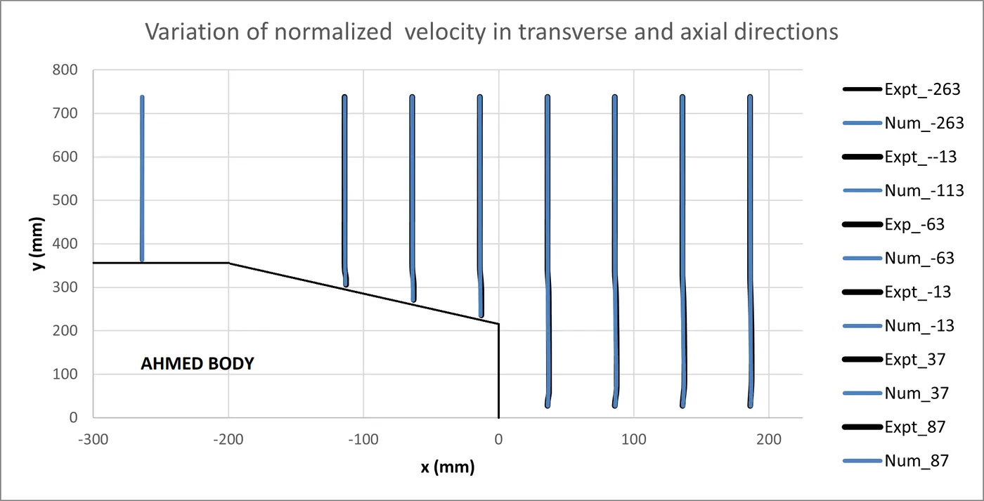
The accuracy of the simulations is verified by comparing the magnitude of the axial velocity obtained at different axial and vertical coordinates experimentally and numerically. A normalized plot has also been created for the reader's convenience. The close agreement between the experimentally and numerically obtained values verify the accuracy of the simulation.
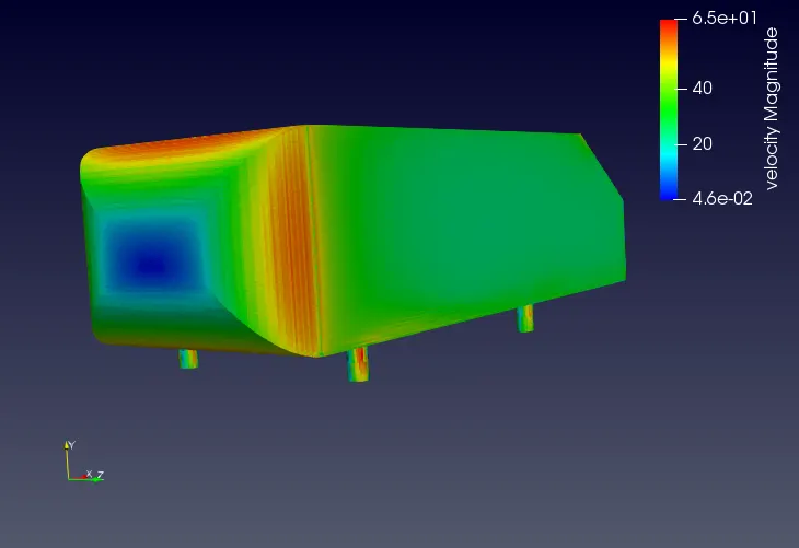
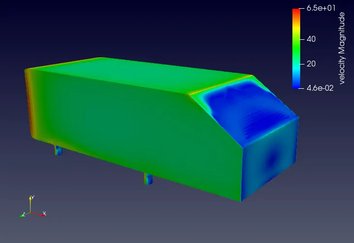
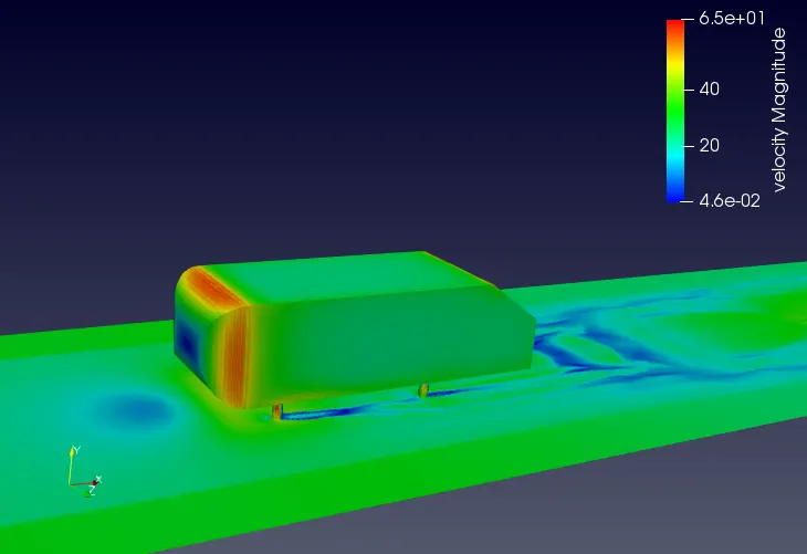
The preliminary observations on the velocity contours are shown below. The downstream portion of the Ahmed Body indicates a significant reduction in velocity, suggesting that the slanting surface of the Ahmed Body might have led to flow separation. There is a noted rise in the velocity along the chamfered edges of the Ahmed Body, which also indicates the presence of flow separation. The sudden loss in velocity at the windward/upstream portion of the Ahmed Body is attributed to the loss of the kinetic energy of the wind, which is converted into one of the major components of the drag force exerted on the body.
Refined mesh: Velocity contours
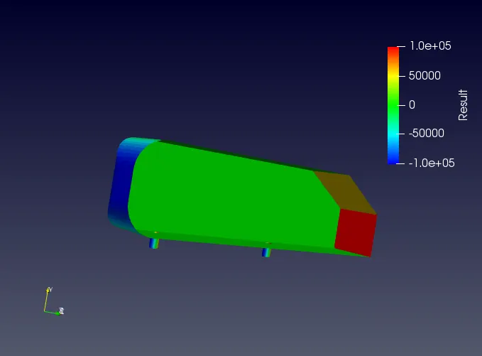
(Contours of drag force)
Furthermore, the lower velocity on the leeward portion of the Ahmed Body suggested the presence of vortices and/or recirculation. The streamline plots shown below confirm the validity of this hypothesis. As a result, the vortices generate a negative pressure/suction component, which exerts further drag on the body. As seen from the drag force contours below, a significant portion of the drag force is exerted from the leeward side as well.
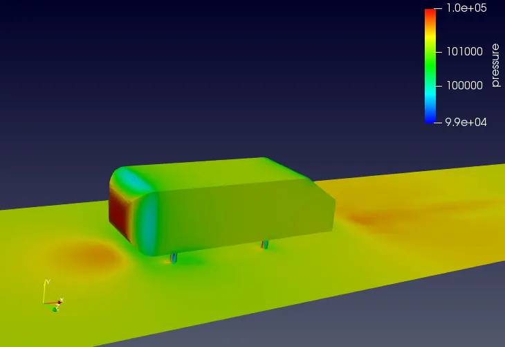
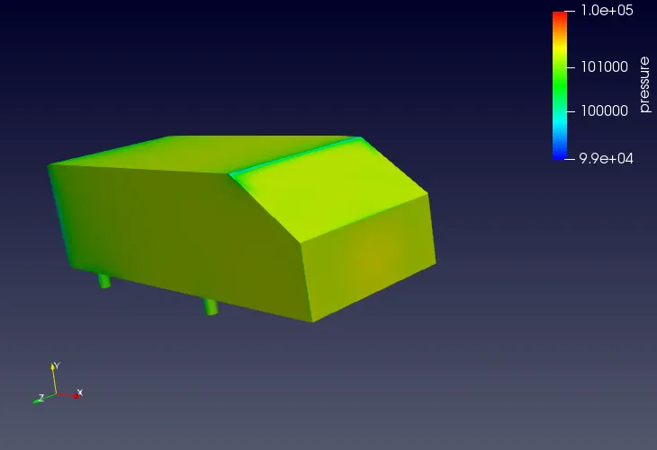
The pressure contours present further interesting hypotheses. The absence of a high pressure region at the bottom of the Ahmed body suggests the presence of a strong downforce and the absence of a lift force. This feature can be attributed to the geometry of the body, which is designed to generate a downforce and keep it in contact with the ground.
Refined mesh: Pressure contours
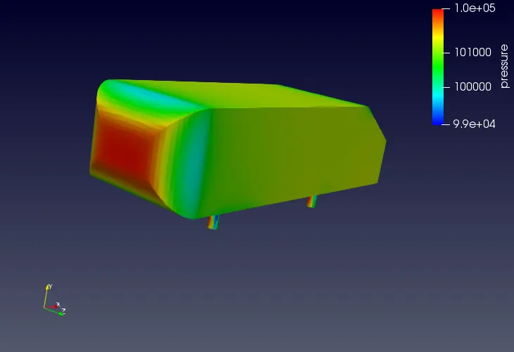
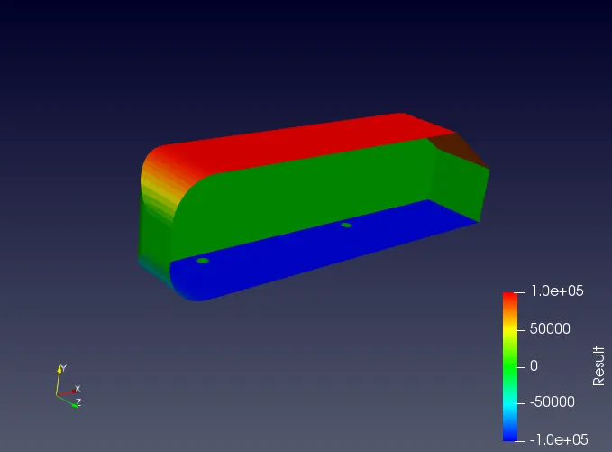
(Contours of Lift/Downforce)
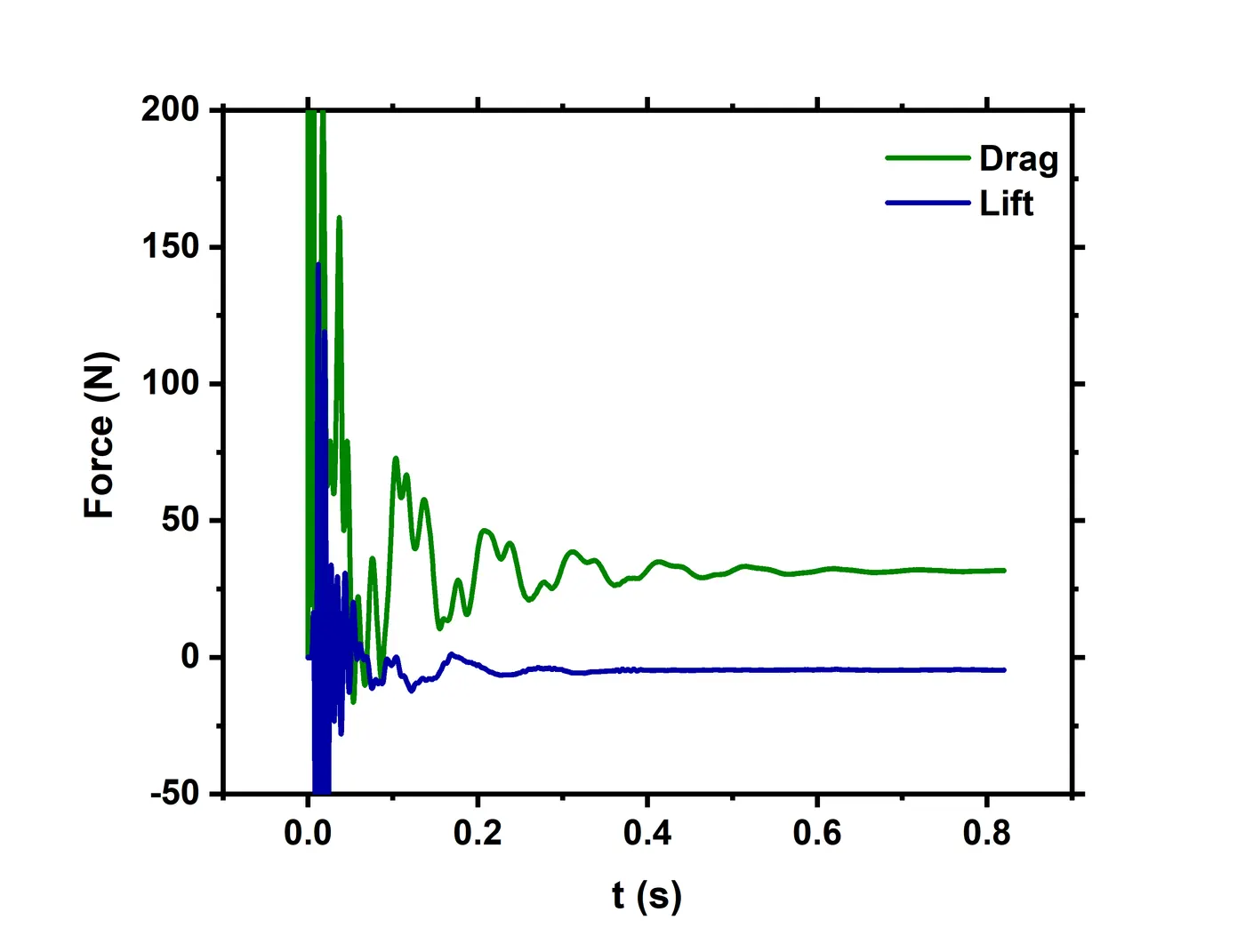
The variation of the average drag and lift forces with time is plotted below. An average drag force of ~31 N and a lift force of ~-4.6 N is reported. Please note that since these simulations were carried out on a coarse mesh, there might be slight deviation between the numerically reported and experimentally obtained values. The calculation for the drag and lift coefficients is shown below.
By using eqns. i and ii, Cd and Cl are calculated as follows
`Cd=(2*D)/((rho*A*v^2)` = `(2*31.6)/((1.17*0.288*0.389*40^2))=0.301`
`Cl=(2*L)/((rho*A*v^2)`= `(2*4.6)/((1.17*0.288*0.389*40^2))=0.044`
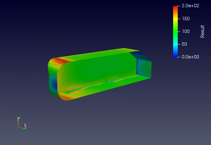
For every CFD simulation, it is crucial to keep a track of the Y+ values. Studying flow separation and wall forces requires the application of a turbulence model which is proven to generate accurate results in the viscous sub-layer and the buffer regions, i.e. 10<Y+<300. Contours of the Y+ values are shown below. Maximum values in the range of ~200 are reported only in regions of high velocity and flow separation. Integrating this value over the entire surface generates a value of 83.82. Since the `k-omega` SST model is proven to be accurate for Y+<300, it is chosen as the turbulence model for the current simulation.
Conclusion
A numerical analysis of the standard Ahmed Body has been carried out in the current study. Clear evidence of flow separation and recirculation has been observed--both of which significantly contribute to the drag and downforce generated. It is crucial to strike a balance between a minimal drag force and a maximum downforce. The drag and lift coefficients have been calculated to be equal to and respectively. Furthermore, the average Y+ value is found to be 83.82, thereby confirming the choice of the turbulence model as the `k-omega` SST model