3D CFD analysis of thermal mixing in a T junction

Aim – Three dimensional CFD analysis of turbulent mixing of hot and cold fluid streams in T - junction using Ansys 2020 R2.

Introduction –

The turbulent mixing problem is one of the most studied CFD problems, both computationally and experimentally. Its applications are widespread in the chemical, petrochemical, HVAC and other industries. One of the most common household application is the mixing of hot and cold water streams, probably available in all the houses.

In industrial applications, it is most widely used in the HVAC industry to get an optimum temperature in a living space. The cold stream of air from the air conditioning system can be mixed with the ambient air to get a desired temperature. The desired temperature can be controlled by varying the mass flow rates of the streams.

Thus, due to its wide applications a computational study has been performed in the present work using Ansys Fluent Student Version (Version 2020 R2).

Modelling and Solving approach –

1. Solid Model – A 3D CAD model was already provided. This CAD model was imported in Ansys Spaceclaim. A volume extraction was then performed to get the domain of study. Two different pipe configurations have been used. The difference is in the length between the secondary inlet and the exit of the main pipe. Both configurations are shown below –

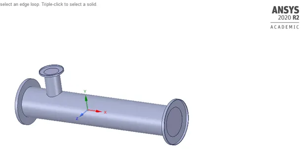
Figure 1. 3D CAD model (Short pipe) imported in Ansys Spaceclaim.

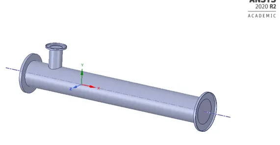
Figure 2. 3D CAD model (long pipe) imported in Ansys Spaceclaim.

2. Meshing – Ansys Meshing was used to create the mesh using tetrahedral elements for a simple study. The mesh details have been provided in the subsequent sections.
3. Solver Settings – Ansys Fluent was used as the solver. A steady state computational study has been performed using a pressure based solver. Air was used as the fluid entering from both the inlets. The default physical properties defined in Fluent were used.
4. Boundary conditions – Momentum ratio of 2 and 4 have been used in the study. The hot stream enters in the main pipe (larger diameter) while the colder stream enters from the secondary inlet. The boundary conditions are given below in Table 1 –

Table 1. Boundary conditions

	Velocity of hot air stream (m/s)	Velocity of cold air stream (m/s)	Temperature of hot air stream (oC)	Temperature of cold air stream (oC)
Case 1	3	6	36	19
Case 2	3	12	36	19

1. Computational model – A comparative study between k omega SST and Realizable k epsilon models was performed on the short configuration pipe at momentum ratio of 2 and it was concluded that the realizable k epsilon model gave faster convergence and accurate results. Thus, this model was used for all the computations.
2. Spatial Discretization Method – Coupled Pressure velocity coupling scheme was used to solve the Navier Stokes Equations. The methods used for spatial discretization of each of the terms is given in the below table –

Table 2 Spatial discretization Methods used

Term/Equation	Method
Gradient	Least Squares Cell based
Pressure	Second Order
Momentum	Second Order Upwind
Turbulent Kinetic Energy	First Order Upwind
Turbulent dissipation Rate	First Order Upwind
Energy	Second Order Upwind

4. Results and Discussion –

The analysis has been performed on both the short and long pipe configurations for different momentum ratios. Momentum ratio (MR) is defined as –

Where v_h is the velocity of hot fluid stream while v_c is the velocity of cold fluid stream.

The boundary conditions have already been listed in Table 1 above.

Case 1 – The momentum ratio is chosen as 2.

Short pipe configuration -

The meshed short pipe geometry and element quality metric are shown below.

A mesh independence test has also been performed. The results are given in Table 3 below. K-omega SST model has been chosen for this test.

Table 3 Mesh Independence test

Number of elements	Element size (m)	Area weighted average of Temperature at outlet (oC)	Standard deviation of temperature at outlet (oC)	Iterations for convergence
14247	5e-03	30.25	2.0	212
39817	3e-03	30.30	2.30	262
105858	2e-03	30.40	2.30	263

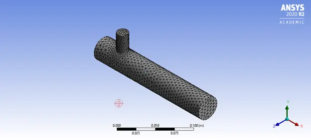
Figure 3 Meshed geometry with element size of 5e-03.

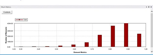
Figure 4 Element metrics when element size is 5e-03

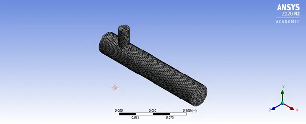
Figure 5 Meshed geometry with element size of 3e-03.

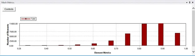
Figure 6 Element metric when element size is 3e-03.

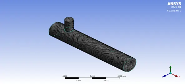
Figure 7 Meshed geometry with element size of 2e-03.

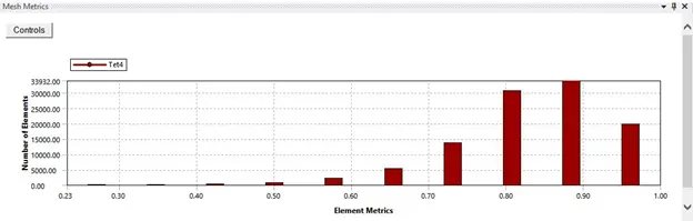
Figure 8 Element metric when element size is 2e-03.

Since the area weighted temperature at the outlet face nearly same for all the mesh sizes, element size of 3e-03 has been chosen on the basis of standard deviation at the outlet face.

The residual, area weighted temperature and standard deviation plots are shown below for all the three element size mentioned in Table 3.

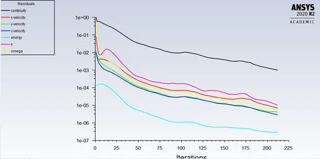
Figure 9 Residual plot when element size is 5e-03 using k-omega-SST model.

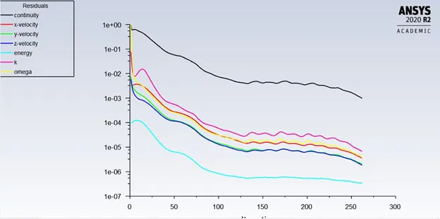
Figure 10 Residual plot when element size is 3e-03 using k-omega-SST model.

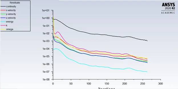
Figure 11 Residual plot when element size is 2e-03 using k-omega-SST model.

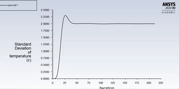
Figure 12 Standard deviation plot when element size is 5e-03 using k-omega-SST model.

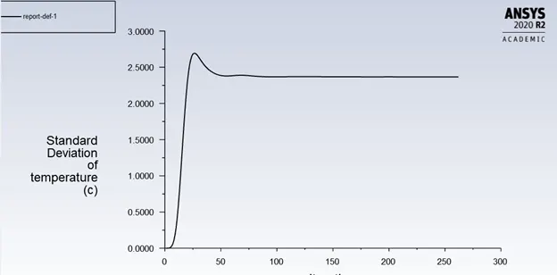
Figure 13 Standard deviation plot when element size is 3e-03 using k-omega-SST model.

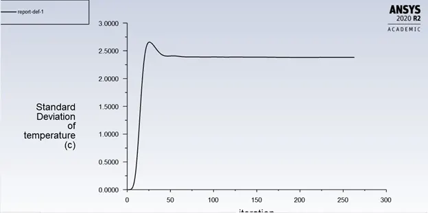
Figure 14 Standard deviation plot when element size is 2e-03 using k-omega-SST model.

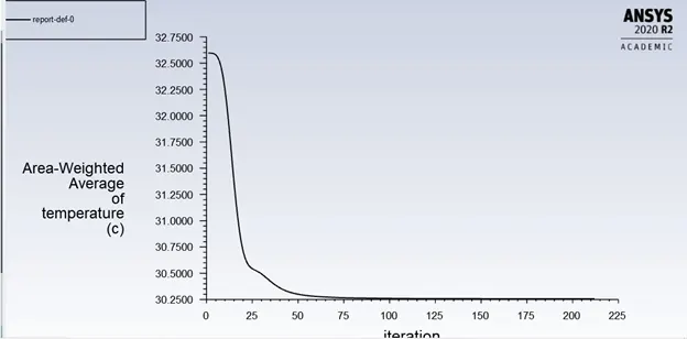Figure 15 Area weighted average of temperature at outlet when element size is 5e-03 using k-omega-SST model.

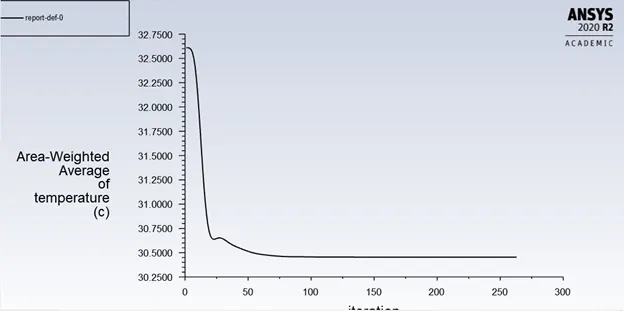
Figure 16 Area weighted average of temperature at outlet when element size is 3e-03 using k-omega-SST model.

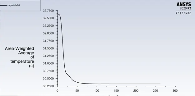
Figure 17 Area weighted average of temperature at outlet when element size is 2e-03 using k-omega-SST model.

The standard deviation is an indicator of the mixing efficiency achieved. From the above plots of standard deviation, it is clear that the mixing efficiency achieved for this configuration is less (due to higher standard deviation values). Also, the temperature at the outlet face is quite high. Mixing efficiency can be improved by using a longer pipe. This has been shown below. While a lower temperature can be achieved by increasing the velocity of cold fluid which forms the basis of Case 2.

The below velocity and temperature contours and line plots are shown only for element size of 3e-03 using the k – omega – SST model.

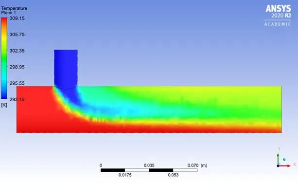
Figure 18 Temperature contour.

It is evident from the temperature contour plot that most of the diffusion occurs near the junction and also due to the lower momentum of the cold stream, the hot stream dominates and therefore, the mixture is at slightly higher temperature.
The temperature line plot in Figure 19 indicates that there is sudden temperature drop just near the T junction. However, this temperature rises as the distance along the pipe length increases due to heat transfer from the cold to the hot fluid.

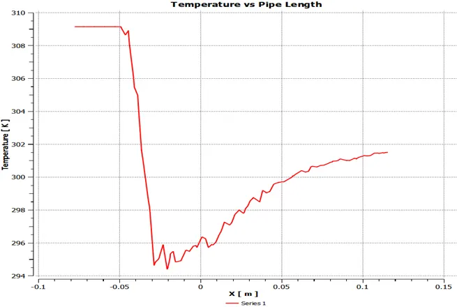Figure 19 Temperature along the center line of the pipe.

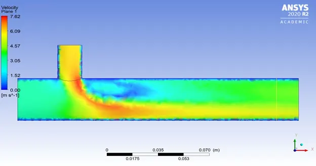
Figure 20 Velocity contour plot

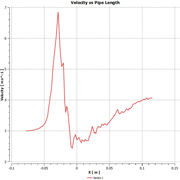
Figure 21 Velocity along the centerline of the pipe

The velocity contour plot highlight a recirculation zone developed near the T junction on the upper boundary of the domain as both the fluid streams try to mix with one another. Also, the velocity is slightly higher near the T junction because the hot fluid (at lower velocity) tends to push the colder fluid due to momentum transfer. The same is indicated in the line plot above.

k-omega-SST vs Realizable k-epsilon model

The above analysis has been performed using the k-omega-SST model. Another model available in Fluent and widely used is the k-epsilon model. Thus, the same analysis was again carried out using Realizable k-epsilon model with standard wall functions. Both the models have their advantages and disadvantages. The k-omega model is better for near wall boundary layer modelling while the k – epsilon model gives better results for flows where separation is not a concern. However, the solution by k-epsilon may suffer by instabilities due to numerical diffusion. The same has been observed in the analysis (refer residual plot below). However, since we are concerned with the temperature at the outlet of the pipe and the k-epsilon model gives faster convergence, thus, further studies have been performed using the k-epsilon model.

The results using k-epsilon model are given below.

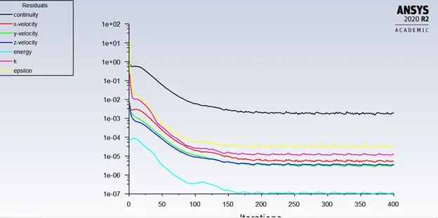
Figure 22 Residual plot using k-epsilon model

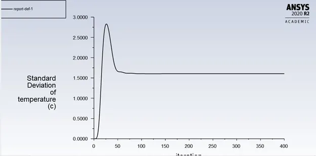
Figure 23 Standard deviation using k – epsilon model

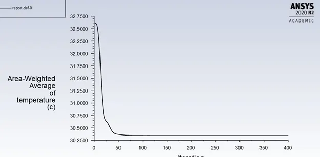
Figure 24 Area weighted average of temperature using k – epsilon model

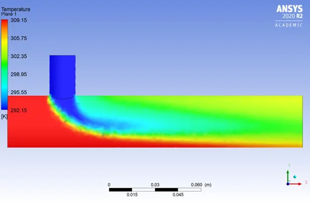
Figure 25 Temperature contour using k-epsilon model

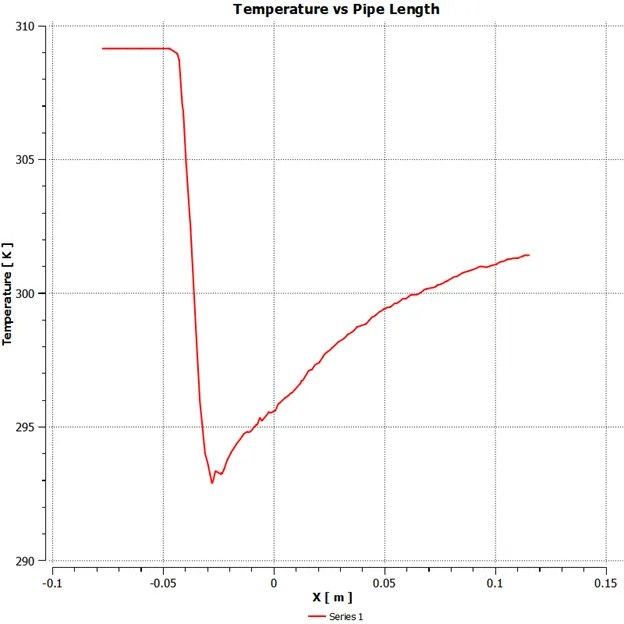
Figure 26 Temperature along the centerline of the pipe using k-epsilon model

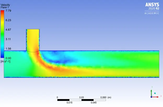
Figure 27 Velocity contour using k-epsilon model

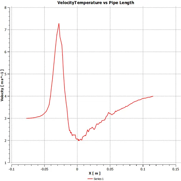
Figure 28 Velocity along the centerline using k-epsilon model

Long Pipe configuration-

The long pipe configuration is now analyzed for the same momentum ratio with an element size of 3e-03 m. A mesh independence test has also been perform for this configuration using element size of 3e-03 m and 2e-03 m. Element size of 3e-03 m has been chosen. The residuals, area weighted temperature, standard deviation, velocity and temperature contour plots for the same mesh (element size 3e-03 m) are shown below.

Table 4 mesh independence test for long pipe configuration

Number of elements	Element size (m)	Area weighted average of temperature at outlet (oC)	Standard deviation of temperature at outlet (oC)
56526	3e-03	30.3	1.25
141588	2e-03	30.3	1.25

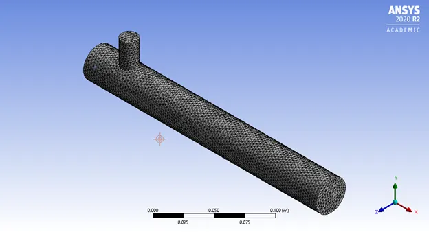
Figure 29 Meshed pipe with element size of 3e-03 m.

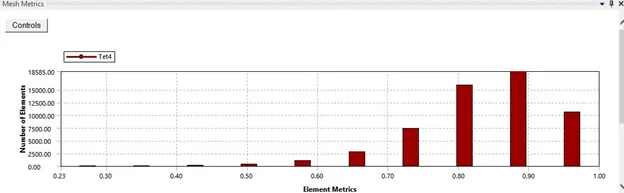
Figure 30 Element metric for long pipe configuration with element size of 3e-03 m.

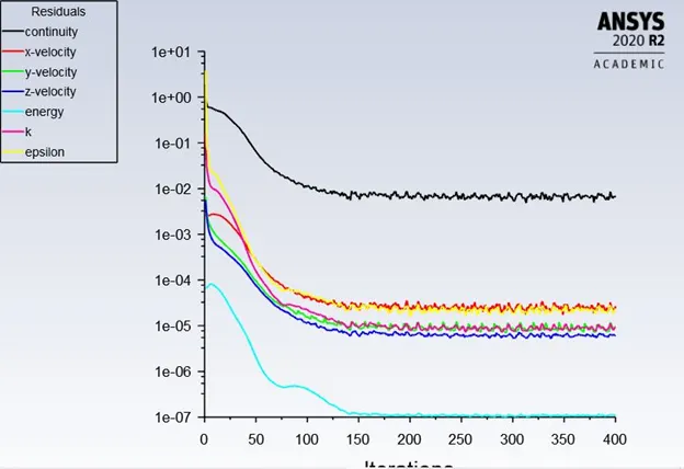
Figure 31 Residual plot for long pipe configuration

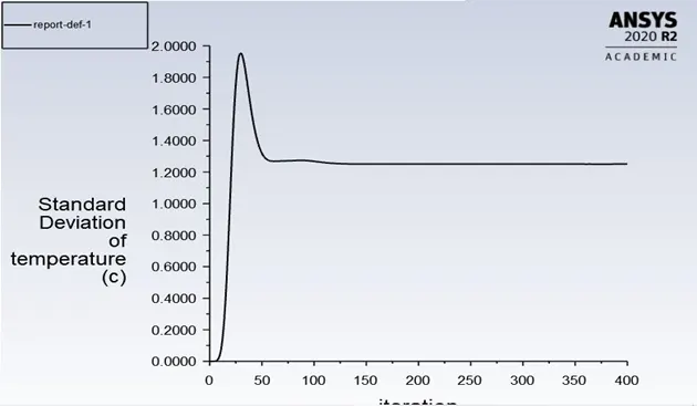
Figure 32 Standard deviation plot

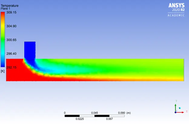
Figure 33 Temperature contour

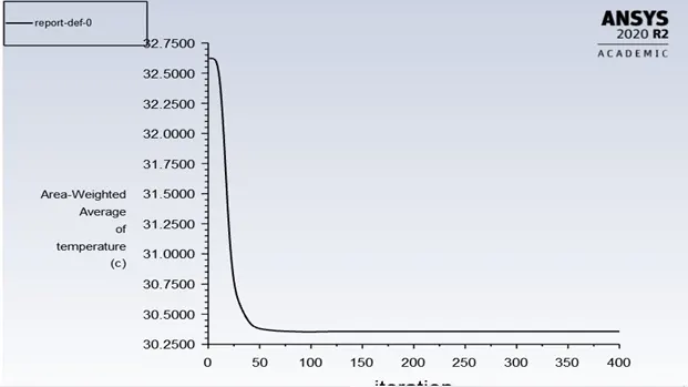Figure 34 Area weighted average of temperature at outlet face

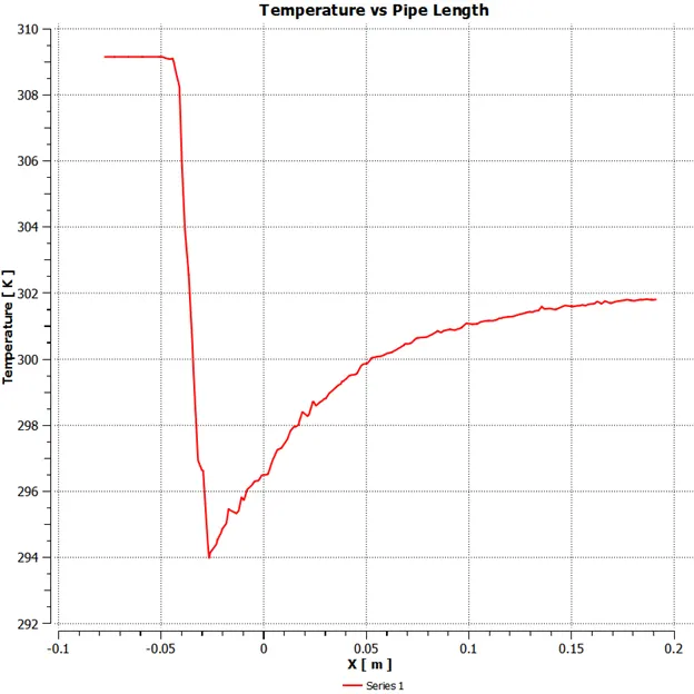
Figure 35 Temperature along the centerline

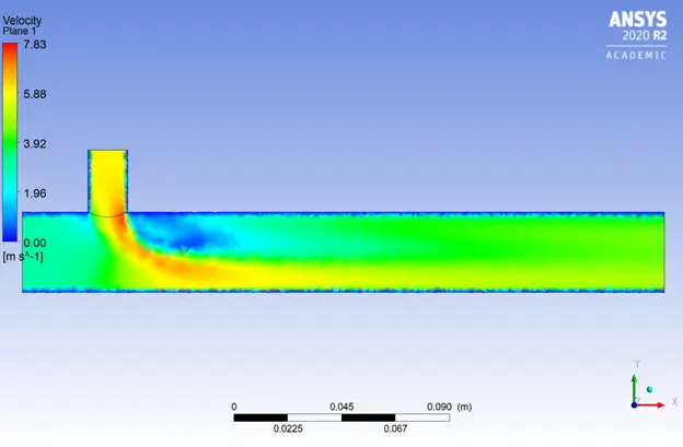
Figure 36 Velocity contour

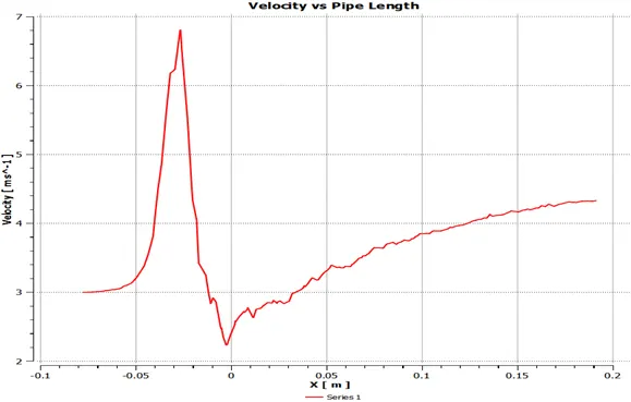
Figure 37 Velocity along the centerline

It can be clearly concluded from the standard deviation plot that the long pipe configuration has a higher mixing efficiency. The average temperature at the pipe outlet remain nearly the same. This is because the pipe is adiabatic, thus it doesn’t lose heat as the length of the pipe is increased. Below is the summary of the results obtained.

Table 5. Summary of the results for momentum ratio of 2.

Configuration	Turbulence model	Iterations for convergence	Area weighted average of temperature at outlet (oC)	Standard deviation of temperature at outlet (oC)
Short Pipe	k-omega-SST	262	30.3	2.3
Short Pipe	Realizable k-epsilon	178	30.3	1.6
Long Pipe	Realizable k-epsilon	170	30.3	1.25

Case 2 –

The same analysis has been performed for MR of 4 and the results are given in the below table.

Table 6 Summary of results for momentum ratio of 4.

Configuration	Turbulence model	Iterations for convergence	Area weighted average of temperature at outlet (oC)	Standard deviation of temperature at outlet (oC)
Short Pipe	Realizable k - epsilon	156	27.5	1.1
Long Pipe	Realizable k - epsilon	229	27.5	0.73

When the momentum ratio is increased, the final temperatures at the outlet decrease for both the configurations. However, the standard deviation of the longer pipe is lower which indicates a better mixing efficiency achieved. The same was observed in Case 1.

Short Pipe –

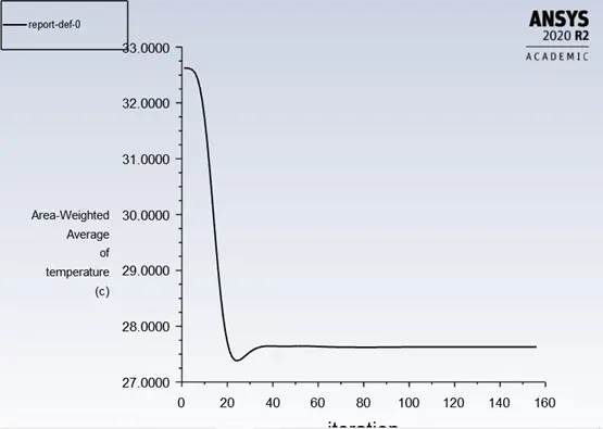
Figure 38 Area weighted average of temperature for short pipe configuration

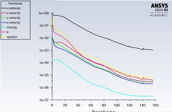
Figure 39 Residual for short pipe configuration

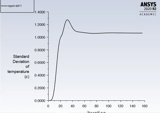
Figure 40 Standard deviation of temperature for short pipe configuration

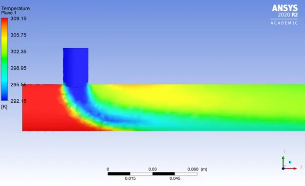Figure 41 Temperature contour

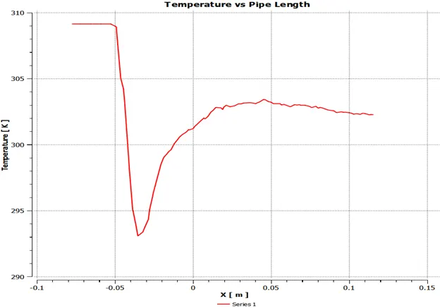
Figure 42 Temperature along the centerline

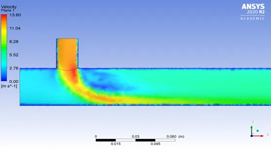
Figure 43 Velocity contour

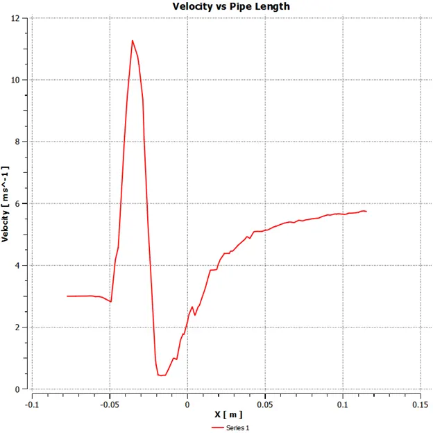
Figure 44 Velocity along the centerline

Long Pipe –

The plots of the results for long pipe configuration are given below. It is clearly evident from the standard deviation plots that longer pipe gives better mixing efficiency as compared to shorter pipe.

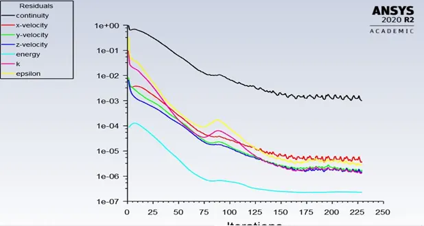
Figure 45 Residual plot for long pipe configuration

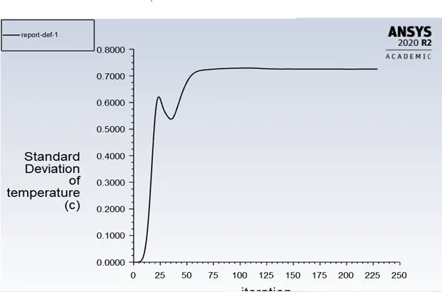
Figure 46 Standard deviation for long pipe configuration

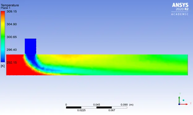
Figure 47 Temperature contour

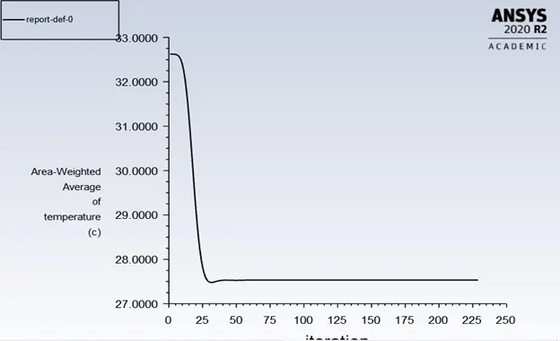
Figure 48 Area weighted average of temperature

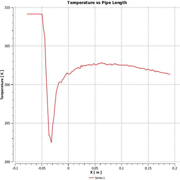
Figure 49 Temperature along the centerline

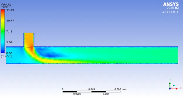Figure 50 Velocity contour

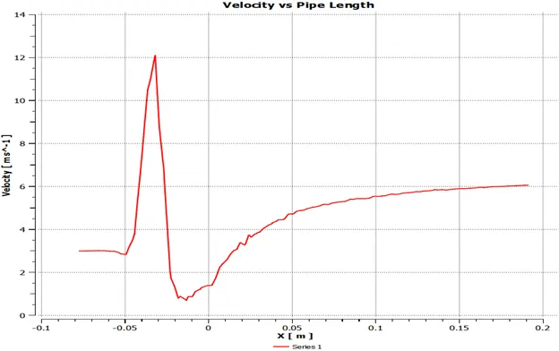
Figure 51 Velocity along the centerline

The below table highlights the important results of both the cases –

Table 7 Summary of results

	Pipe Configuration	Number of elements	Iterations for convergence	Average outlet temperature(oC)
Case 1 (Momentum Ratio = 2)	Short pipe	39817	178	30.3
	Long pipe	56526	170	30.3
Case 1 (Momentum Ratio = 2)	Short pipe	39817	156	27.5
	Long pipe	56526	229	27.5

5. Conclusions

A 3D CFD analysis using Ansys 2020 R2 (Academic) has been performed in the present analysis. The effect of length of the pipe and momentum ratio has then been studied.

It can be clearly concluded from the CFD analysis that long pipe configuration achieves much better mixing efficiency (indicated by standard deviation). The lower the standard deviation, the better the mixing efficiency. Thus, the mixing efficiency is directly proportional to the length of the pipe. Also, the higher the momentum ratio, the lower will be the temperature at the pipe outlet. This can be attributed to the higher velocity of the cold fluid thereby increasing its momentum. The momentum and thereby energy transfer from cold high speed fluid to hot low speed fluid results in lower temperature of the mixture at pipe exit.