Mixing efficiency

For this challenge, we have created two versions of the mixing tee. One of them is longer than the other.

Your job is to set up steady-state simulations to compare the mixing effectiveness when the hot inlet temperature is 36⁰C & the Cold inlet is at 19⁰C.

Use the k-epsilon and k-omega SST model for the first case and based on your judgment use the more suitable model for further cases. Giving the reason for choosing a suitable model is compulsory.

1. Case 1
   • Short mixing tee with a hot inlet velocity of 3m/s.
   • Momentum ratio of 2, 4.
2. Case 2
   • Long mixing tee with a hot inlet velocity of 3m/s.
   • Momentum ratio of 2, 4.

Momentum ratio = velocity at cold inlet / velocity at hot inlet

In a table, compare the following values from the 2 cases.

1. Cell count
2. Average outlet temperature
3. Number of iterations for convergence

Solution:

Aim

Simulation of heat transfer through a T joint pipe using ANSA Fluent

Objective:

To simulate heat transfer in T joint pipe and study the mixing efficiency of fluid, this is achieved by studying the temperature at the outlet of pipe with various lengths and momentum ratio of cold inlet and hot inlet

Mesh independent test

To find out suitable mesh size for our simulation, we need to perform a mesh independent test

Conditions:

Fluid - air

Hot inlet temperature - 36-degree Celcius

Hot inlet velocity - 3 m/s

Cold inlet temperature - 19-degree Celcius

Momentum ratio = 2

Momentum ratio = velocity at cold inlet/velocity at hot inlet

Cold inlet velocity - 6 m/s

`T_(mixture) = (m_(hot)*T_(hot)+m_(cold)*T_(cold))/(m_(hot)+m_(cold))`

The analytical value for T_out = 30.326-degree celsius

Mesh size in mm	2	3	5	7
Outlet Temp in celsius	30.314	30.287	30.252	30.203
%Error (numerical value ~simulated values)	0.3	0.1	0.24	0.4
Cell Count	106253	39769	14247	12592

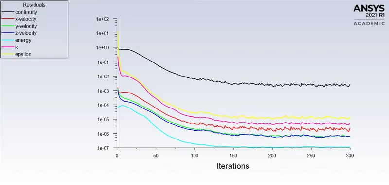
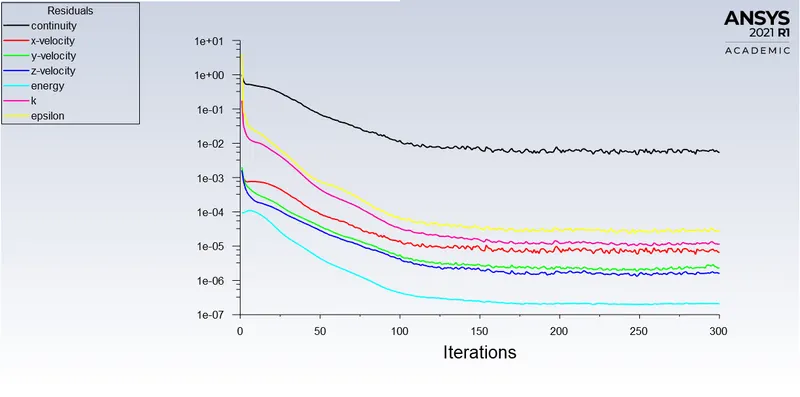
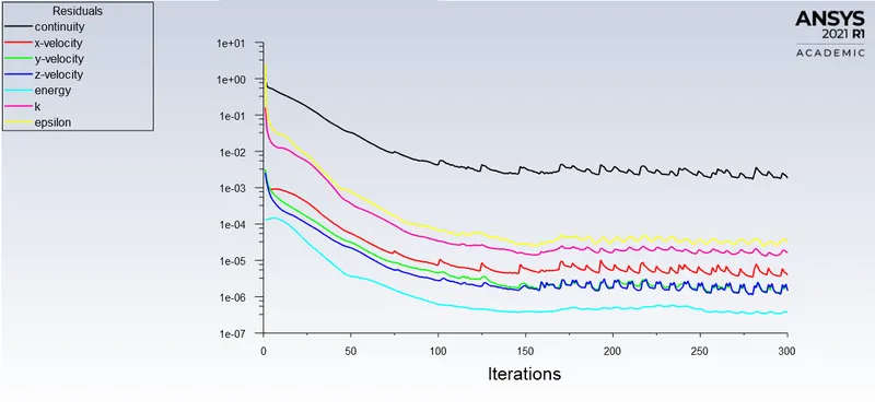
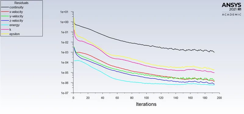
The percentage error must be less than 5% and also we need to see that the system won't longer time to compute the results, as we reduce the mesh size number of elements increase hence the system has to calculate the results at each element.

We need to consider a mesh size that has less percentage error and also considering that the system takes lesser time to compute the results. Here I have considered a mesh size of 3mm.

Residuals

for 2mm

for 3mm

for 5mm

for 7mm

Case-1 Short mixing tee

K-epsilon Realizable

• Short mixing tee with a hot inlet velocity of 3m/s.
• Momentum ratio of 2, 4.

Momentum ratio = velocity at cold inlet/velocity at hot inlet

For Momentum ratio = 2

Velocity at hot inlet = 3 m/s

velocity at cold inlet = 6 m/s

Hot inlet temperature - 36-degree Celcius

Cold inlet temperature - 19-degree celcius

Type K-epsilon turbulence model

Steps:

1. First, we need to launch the Ansys workbench

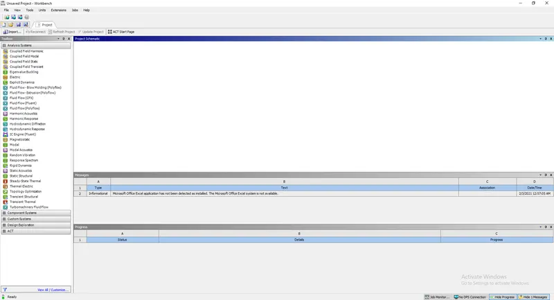
2. In Toolbox select Fluid Flow (Fluent)

3. Now select geometry, Ansys will open Spcaeclaim, which is a CAD platform to generate the geometry

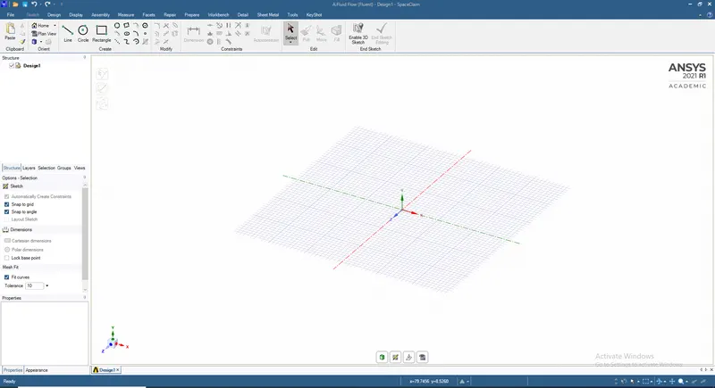
Now import the model to the Spaceclaim environment and extract the volume using the Volume extract tool

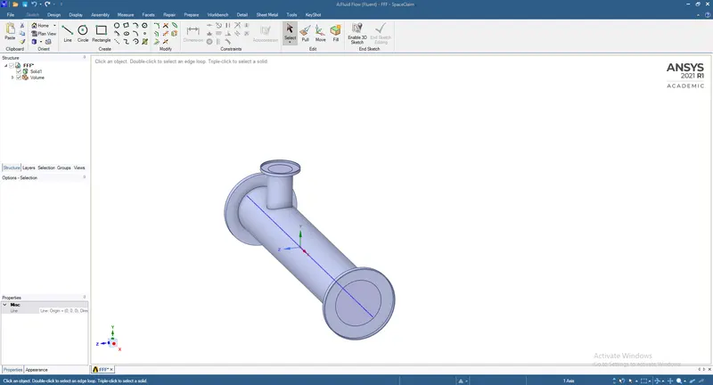
After extracting

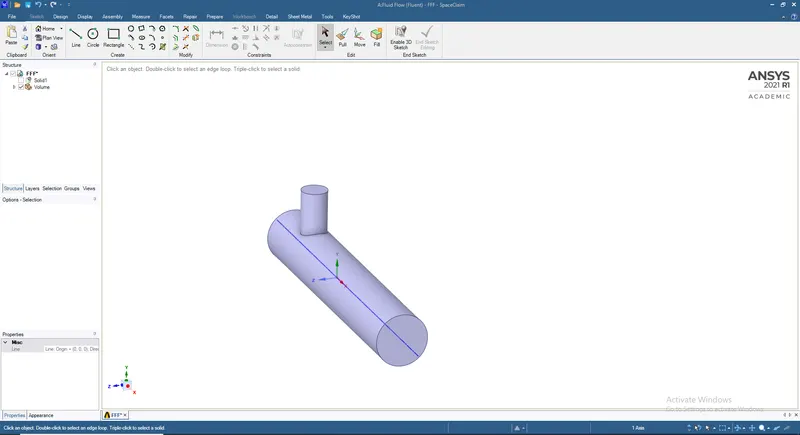
now, close the Spaceclaim

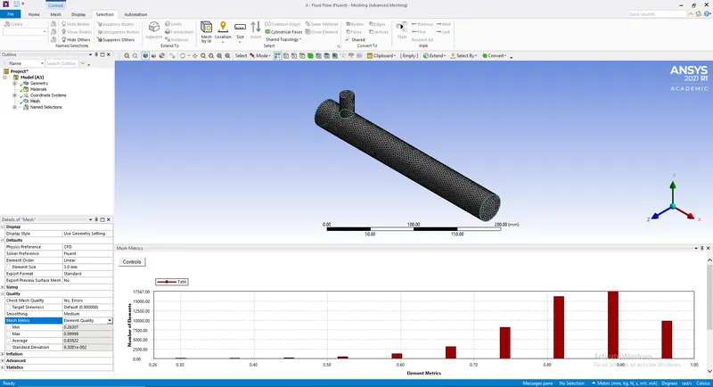
4.Select the Mesh option in the workbench, Ansys will open the Meshing environment, where we need to define mesh size, boundary and check for mesh quality.

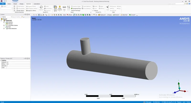
Sizing, boundaries and, mesh quality

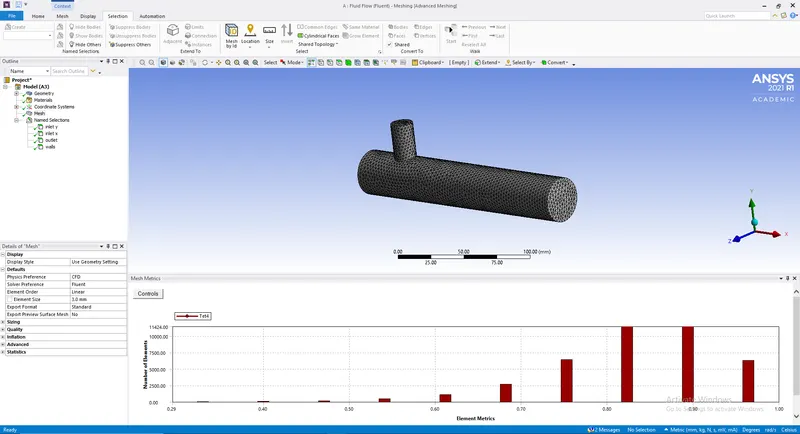
update the mesh and close the meshing environment

5. Now select Setup from the workbench, Ansys will launch Fluent environment

Where we need to define our various simulation conditions, check for mesh quality,

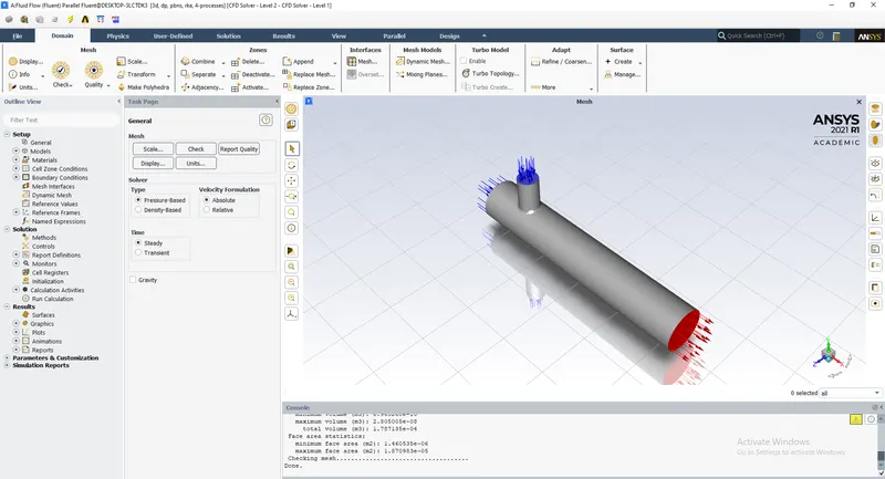
Setting up the physics for our model

where we need to run our simulation in steady-state and defining the boundary parameters in Zones

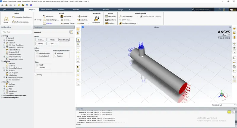
We need to define the type of turbulence model

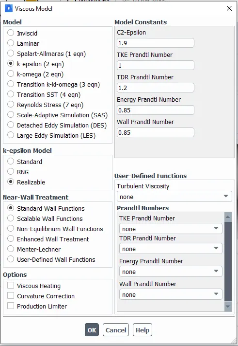
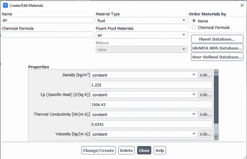
adding material

Now select the solution and click on Initialize

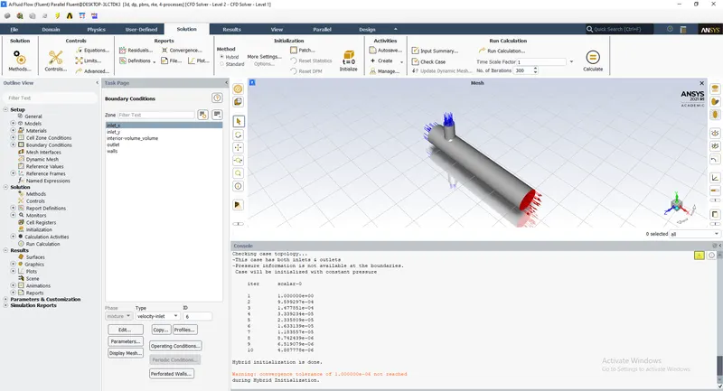
Now enter the number of iterations and hit calculate

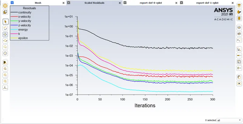
Residuals

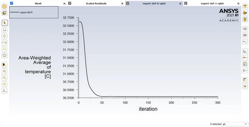
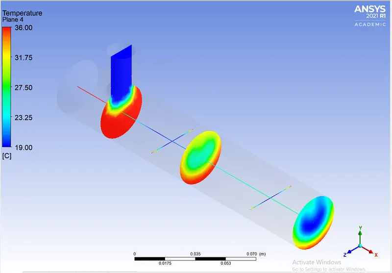
An area-weighted average of Temperature (30.287-degrees Celcius)

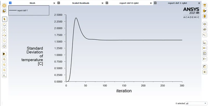
The standard deviation of Temperature (1.55)

Average Outlet temp = 30.287-degree Celcius

number of iterations for convergence 135 to 160

After results are computed, close the fluent environment

6. Now select Results for post-processing

enable the wall and make it transparent for a better understanding of the contour plot

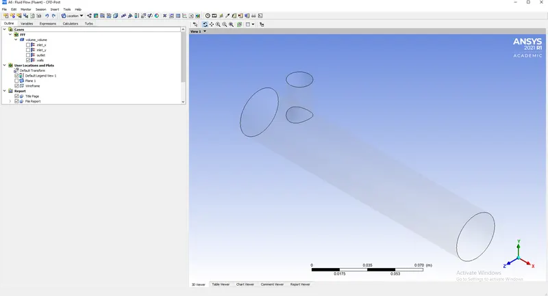
Add plane long XY axis for along the pipe and YZ plane for across the pipe

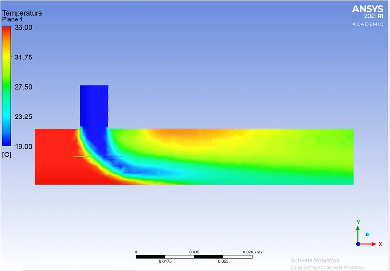
The temperature along the pipe

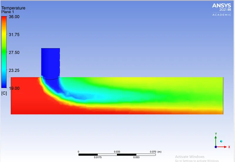
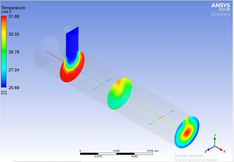
The temperature across the pipe and line plot along the pipe

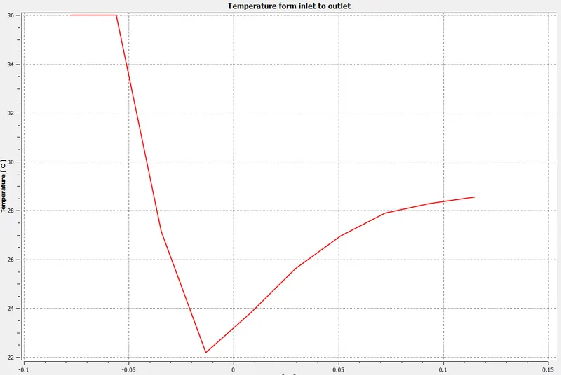
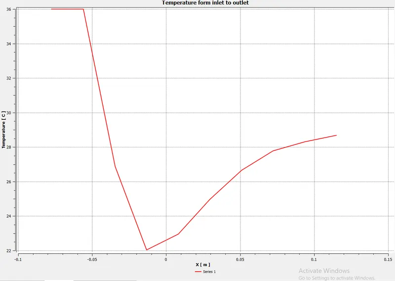
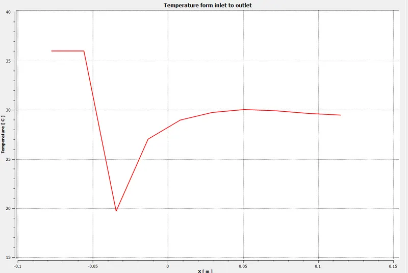
Variation of temperature from inlet to outlet

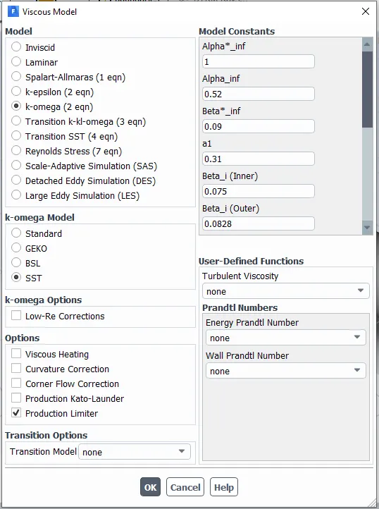
K-omega SST

All the parameters are kept the same, only the Turbulence model is changed to K-omega SST in setup

Residuals

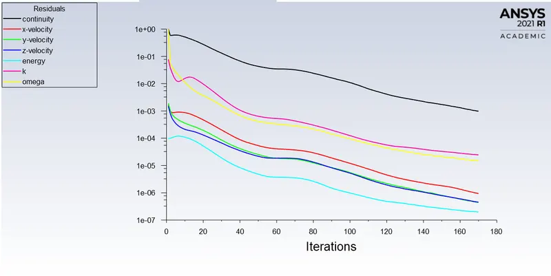
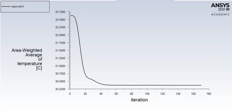
Number of iteration for convergence = 170

An area-weighted average of temperature (30.368-degree Celcius)

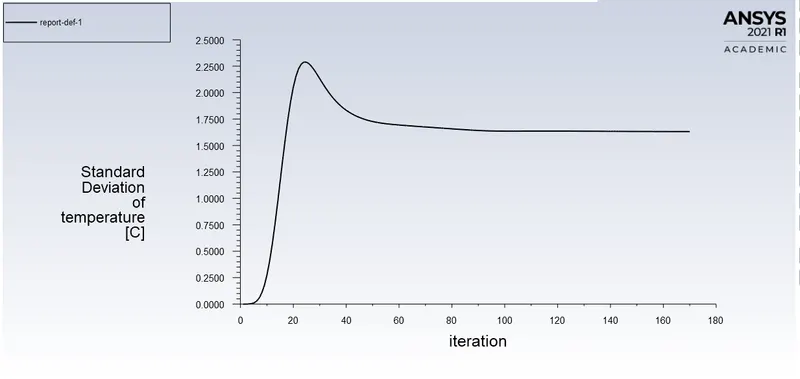
Standard-deviation of temperature (1.63)

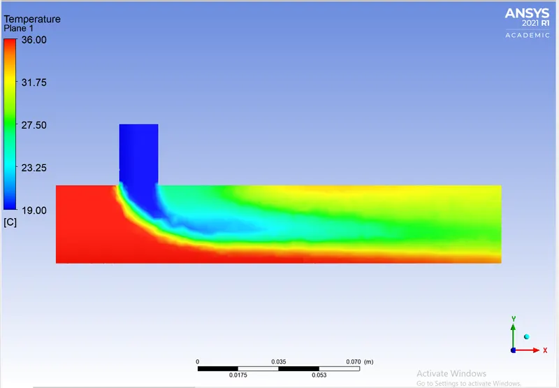
Temperatur along the pipe

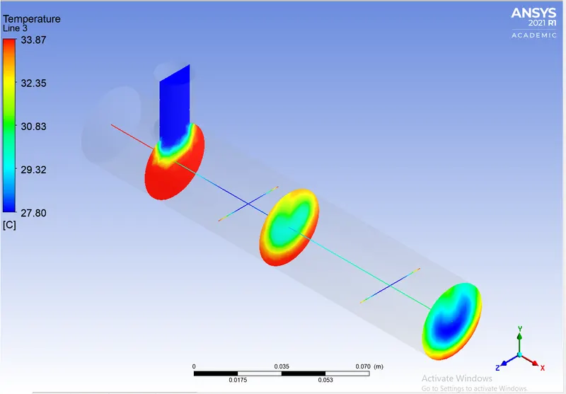
Temperature across the pipe with line plot along and across the pipe

Variation of temperature from inlet to outlet

Comparison of K-epsilon and K-omega turbulence model

Turbulence Model	Average outlet temp in Celcius	Error(30.326 ~ simulated value)	The standard deviation of temp	No of iterations for convergence
K-epsilon Realizable	30.287	0.039	1.55	135-160
K-omega SST	30.368	0.042	1.63	170

From the above table, we can observe that the K-epsilon turbulence model gives the results closer to the analytical value with less percentage of error, it converges at a lesser number of iterations compared to K-omega and shows minimum deviation from the required result.

Hence I have chosen K-epsilon Realizable turbulence model for further cases

For Momentum ratio = 4

Velocity at hot inlet = 3 m/s

velocity at cold inlet = 12 m/s

Hot inlet temperature - 36-degree Celcius

Cold inlet temperature - 19-degree Celcius

The analytical value for T_out = 27.49-degree celsius

Type K-epsilon turbulence model

An area-weighted average of temperature (27.57-degree Celcius)

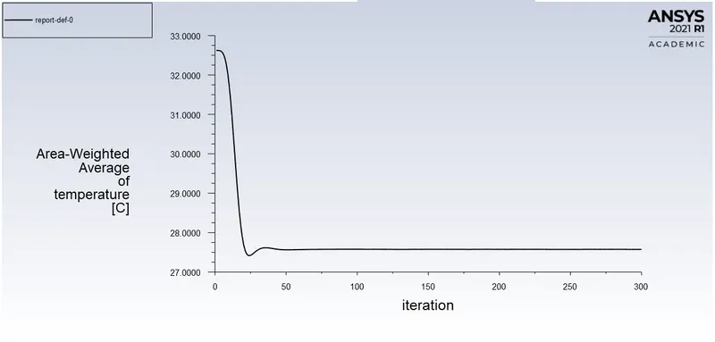
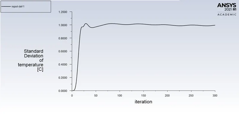
Standard Deviation of temperature (0.99)

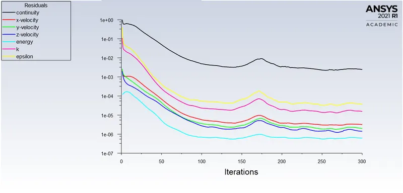
Residuals (convergence at 170 to 220 iterations)

The temperature along the pipe

Temperature across the pipe and Line plot along the pipe

Variation of temperature from inlet to outlet

Case-2 long mixing tee

For momentum ratio = 2

Conditions:

Fluid - air

Hot inlet temperature - 36-degree Celcius

Hot inlet velocity - 3 m/s

Cold inlet temperature - 19-degree Celcius

Momentum ratio = velocity at cold inlet/velocity at hot inlet

Cold inlet velocity - 6 m/s

The analytical value of outlet temperature = 30.326-degree Celcius

Mesh Cell count = 5628 for mess size 3mm

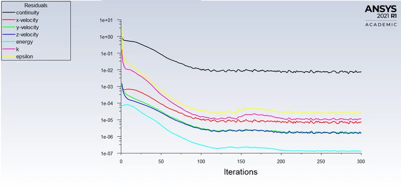
Residuals (converges at 120 to 150 iterations)

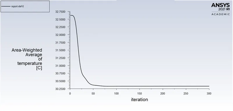
An area-weighted average temperature (30.33-degree Celcius)

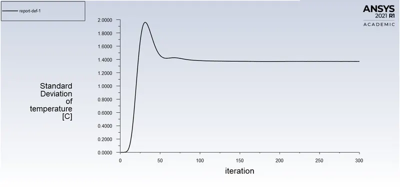
Standard-deviation of temperature (1.36)

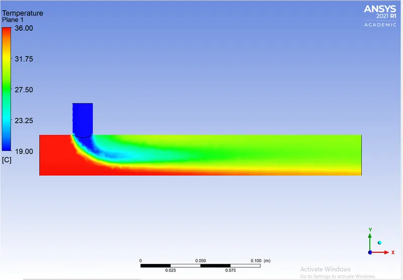
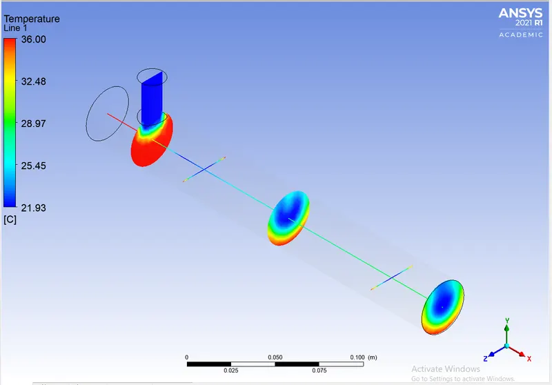
The temperature along the pipe

Temperature across the pipe with line plot along and across the pipe

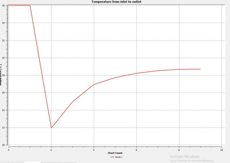
Variation of temperature from inlet to outlet

For Momentum ratio = 4

Conditions:

Fluid - air

Hot inlet temperature - 36-degree Celcius

Hot inlet velocity - 3 m/s

Cold inlet temperature - 19-degree Celcius

Momentum ratio = velocity at cold inlet/velocity at hot inlet

Cold inlet velocity - 12 m/s

The analytical value of outlet temperature = 27.49-degree Celcius

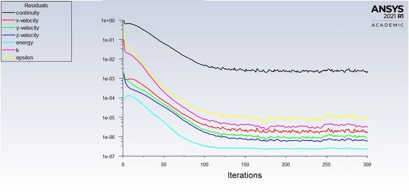
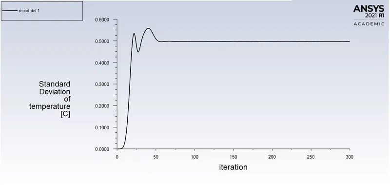
Residuals (converges at 125 to 150 iterations)

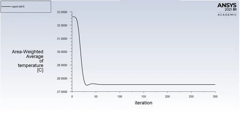
An area-weighted average of temperature (27.52-degree Celcius)

Standard-deviation of temperature (0.49)

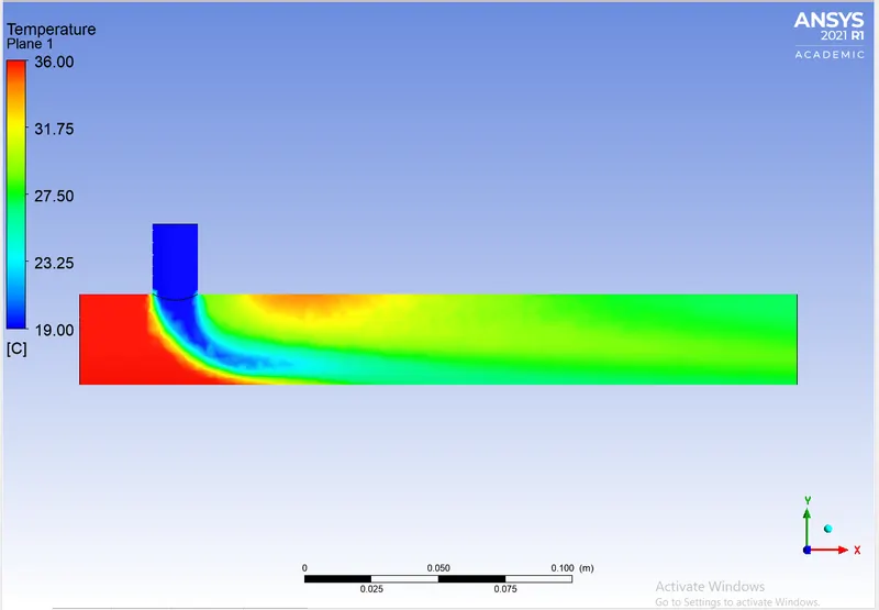
The temperature along the pipe

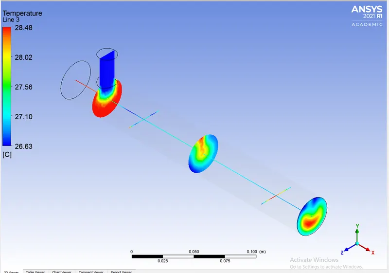
Temperature across the pipe with line plot along and across the pipe

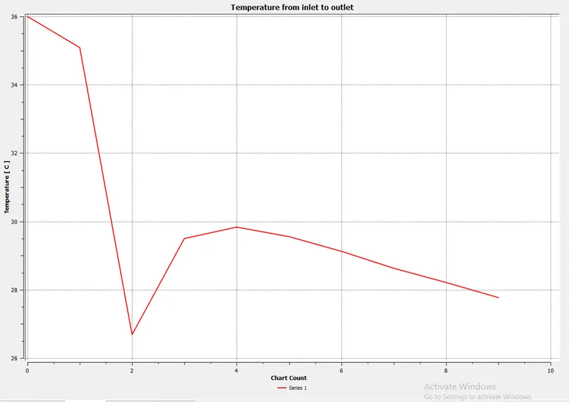
Variation of temperature from inlet to outlet

Comparison Table

Turbulence Model	Momentum Ratio	Analytical value T_out in Celcius	Simulated Value T_out in Celcius	%Error	Standard Deviation	No of iteration for convergence
K-epsilon Realizable Short Tee	2	30.326	30.287	0.12	1.55	135-160
K-omega SST Short Tee	2	30.326	30.368	0.11	1.63	170
K-epsilon Realizable Short Tee	4	27.49	27.57	0.29	0.99	170-220
K-epsilon Realizable Long Tee	2	30.326	30.33	0.01	1.36	125-150
K-epsilon Realizable Long Tee	4	27.49	27.52	0.10	0.49	125-150

By analyzing the table above one can observe that by increasing the velocity of cold air better mixing can be achieved and more uniform flow was observed when the length of the pipe is increased, hence we can see a low standard deviation for temperature.