Mixing efficiency

Mixing Efficiency

1. Introduction, Theory and Aim

A common issue in a pipeline system is the effectiveness of mixing streams, which have different temperatures. CFD simulations help the engineers to predict the heat transfer between the streams and evaluate the outlet velocity and temperature profiles. The theory behind this phenomenon is the conservation of energy, which says that the outlet temperature is equal to the sum of the productions of the inlet temperature and inlet mass for the two entries, divided by the sum of the inlet masses. The aim of this challenge is to investigate the flow field and the heat transfer in a mixing tee, comparing two different configurations (long/short version).

2. Solving & Modelling approach

In order to have a comprehensive understanding of mixing effect, two different T-joins are explored. Both of them have the same inlet boundaries (velocity and temperature) but one of them has more length for the flow to be mixed. This exercise helps us to realise how the outlet temperature varies with the pipe mixing length and different momentum ratios.

3. Pre-processing and solver setting

Import Geometry to the SpaceClaim.

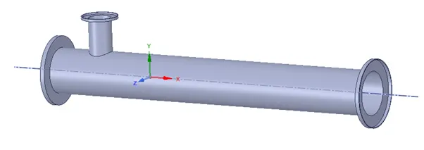
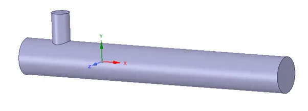
Extract the inside volume and subpress the solid geometry for physical processes.

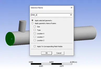
In meshing interface, the geometry is automatically loaded. Then, the faces are selected and given corresponding names (inlet_y, inlet_x, outlet, wall).

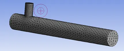
Mesh is automatically generated.

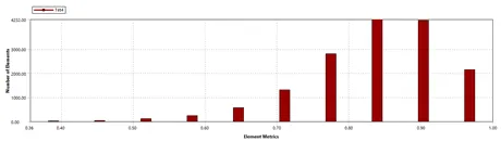
Here we have the quality of the mesh. It can be seen that the majority of the points have element metric more than 0.8.

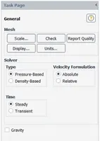
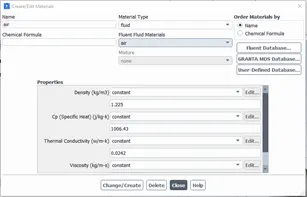
In fluent environment, the solver parameters as well as the material are set.

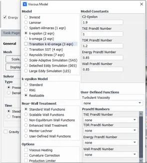
Energy option and k-epsilon realizable viscous model with standard wall functions are selected.

Cell zone conditions and boundary conditions (based on the challenge description) are defined.

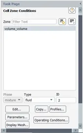
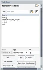
In solution tab, temperature and temperature standard deviation at the outlet were selected to be exported.

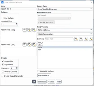
Then, the computational domain needs to be initialised and the solver runs for 500 iterations.

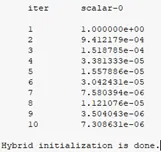
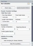
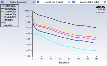
Finally, the simulation converges after 140 iterations.

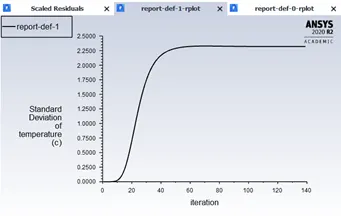
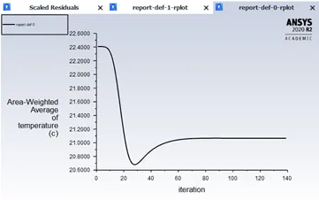
This preparation is done for only one case, but it will be repeated for all the tested cases without giving all these detailed screenshots.

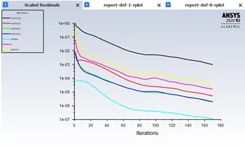
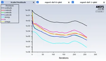
With regards to the different viscous model analysis, we have the following results. The first figure shows that the residual converged after 170 iterations using k-epsilon realizable viscous model, (average temperature: 294.21) while the simulation needs about 260 iterations when k-omega SST viscous model used (average temperature: 294.21). K-epsilon realizable viscous model was selected due to its quicker convergence and better mixing prediction.

4. Results

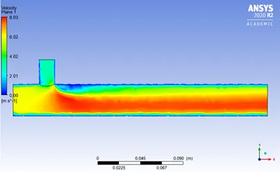
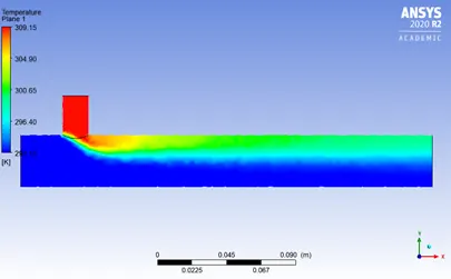
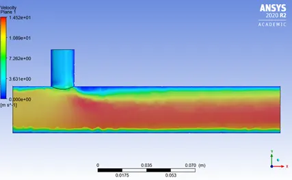
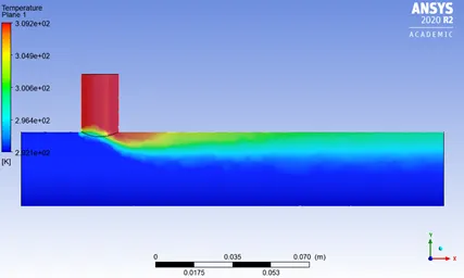
a. Velocity and temperature contour plots on the cut planes along and across the pipe.

- long pipe, momentum ratio 2

- long pipe, momentum ratio 4

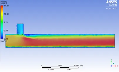
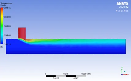
- short pipe, momentum ratio 2

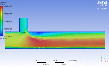
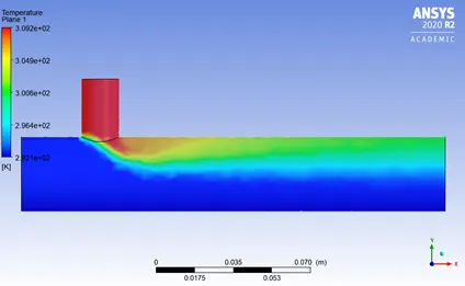
- short pipe, momentum ratio 4

b. In the following table, there is a comparison of the following values from the 2 cases.

Length / Momentum Ratio	Number of Cells	Area-Weighted Output Temperature [K]	Iterations to converge	Area-Weighted Output Temperature STD [K]
Long / 2	17845	294.21	143	2.44
Short / 2	14225	294.31	127	2.9042
Long / 4	17845	293.27	117	1.8328
Short / 4	14228	293.32	138	2.234

c. Perform Mesh independent study for any one case.

In the following table, a mesh independent study can be seen. The result come from a long pipe simulation at momentum rate of 2.

Cell Size [m]	Number of Nodes	Area-Weighted Output Temperature [K]	Area-Weighted Output Temperature STD [K]
5e-3	17845	294.21	2.4404
3e-3	56526	294.2	2.2759
2e-3	141588	294.2	2.2898

The results show that even with 17845 nodes the result is quite accurate.

d. Discuss the effect of length and momentum ratio on results.

It is clear that, in both cases, the higher the momentum ratio, the lower the output temperature and the better the mixing effectiveness. The decrease in temperature is almost 1K and in STD is 0.8K for each case. With regards to the length effect on the results, there is a slight increase in the temperature and the std for the short pipe for all momentum ratio cases. This means that the length does not have a large impact on the mixing effectiveness.

After the tee, the area-weighted average temperature increases due to the hot stream. Then, the mean temperature decreases downstream due to mixing effect. In this simulation the temperature decrease is approximately 0.1K.

5. Conclusion

To conclude, the solution is converged but the effectiveness of the mixing process is not achieved very well because the Area-Weighted Output Temperature Standard Deviation is approximately 2K.

The simulation has been successfully checked for both the grid dependency and for different viscous models.

Finally, it is observed that increasing the length of the mixing part of the pipe does not enhance the mixing effectiveness, while the increased momentum ratio indeed helps.