Matlab Program for OTTO Cycle, finding Thermal Efficiency & making plots for it

Aim:- To write a code that can solve an otto cycle and make plots for it.

• Code to create a PV diagram
• Output the thermal efficiency of the engine.

Introduction:- Air standard cycles are very important, gives us the theoretical limits of a particular cycle which are commonly used in IC engines and Gas Turbines these days.

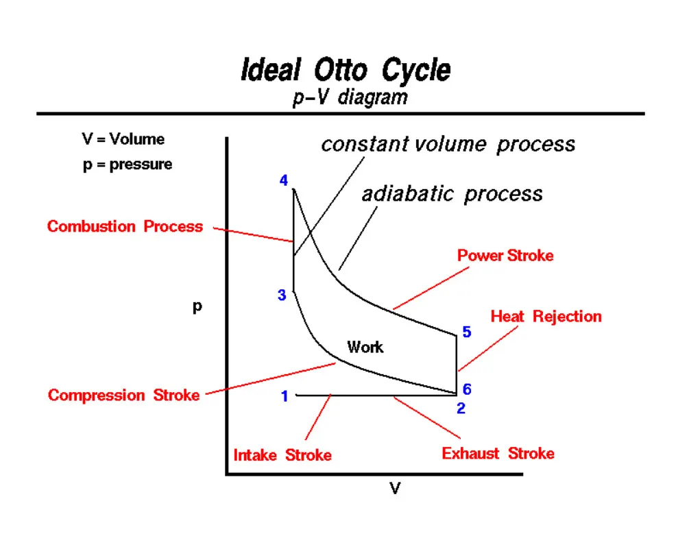
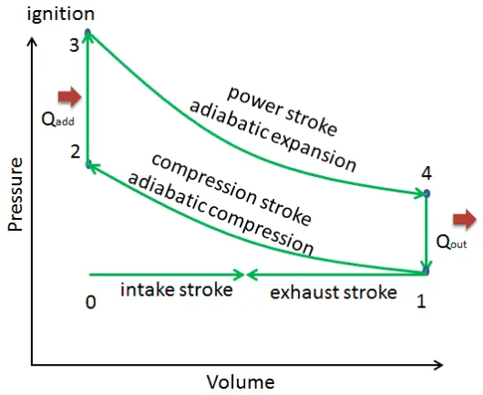
Ideal Otto Cycle:-

Inputs:-

• With V1, T1 we can calculate P1 - Volume(V), Temperature(T) & Pressure(P) at state 1
• With Compression Ratio (Cr) & V2, we can calculate P2, similarly we can calculate T2 - Volume(V), Temperature(T) & Pressure(P) at state 2
• Assume T3, calcute V3 similarly P3 - Volume(V), Temperature(T) & Pressure(P) at state 3
• Similarly T4,V4,P4 are calculated - Volume(V), Temperature(T) & Pressure(P) at state 4, so that we can construct the P-V diagram

Key Points:-

• In order to complete the P-V Diagram, we should know that volume changes from state 1 to state 2.
• It depends on engine kinematics, so we are going with the engine geometric parameters like Bore, Stroke, Connecting Rod Length & Compression Ratio
• Swept volume & clearance volume can be calculated by V1 & V2.
• Swept volume = volume of a cylinder defined by the bore and stroke, Swept Volume = π/4 * bore^2 * stroke
• Clearance volume = Swept volume/ (Cr -1), where Cr is Compression Ratio
• V1 = Swept Volume + Clearance Volume
• V2 = Clearance Volume

Code:-

%inputs 
gamma = 1.4
t3 = 1000

%state variables
p1 = 101325
t1 = 500

%Engine geometric parameters
bore = 0.1;
stroke = 0.1;
con_rod = 0.15;
cr = 12;

% calculating the swept volume and the clearance volume
v_swept = (pi/4)*bore^2*stroke;
v_clearance = v_swept/(cr-1);

v1 = v_swept + v_clearance
v2 = v_clearance

% state variables at state point 2 
%p2v2^gamma = p1v1^gamma
%p2 = p1*(v1/v2)^gamma = p1*cr^gamma

p2 = p1*cr^gamma;

%p1v1/t1 = p2v2/t2   | t2 = p2*v2*t1/(p1*v1)
t2 = p2*v2*t1/(p1*v1);

%state variables at state point 3
v3 = v2

%p3v3/t3 = p2v2/t2 | p3 = p2*t3/t2
 p3 = p2*t3/t2
 
 %state variables at state point 4
 v4 = v1
 
 %p3v3^gamma = p4v4^gamma | p4 = p3(v3/v4)^gamma
 p4 = p3*(v3/v4)^gamma

 hold on
plot(v1,p1, '*',  'color', 'b')
plot(v2, p2, '*',  'color', 'b')
plot(v3, p3, '*',  'color', 'b')
plot(v4, p4, '*',  'color', 'b')

plot ([v1, v2, v3, v4, v1], [p1, p2, p3, p4, p1], 'color', 'r')
xlabel ('Velocity')
ylabel ('Pressure')

Figure & Workspace values:-

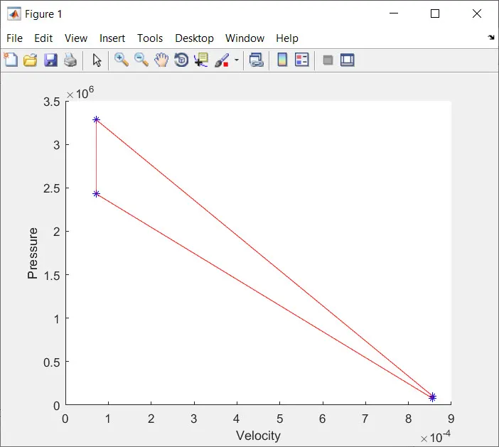
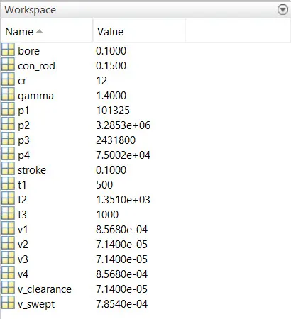
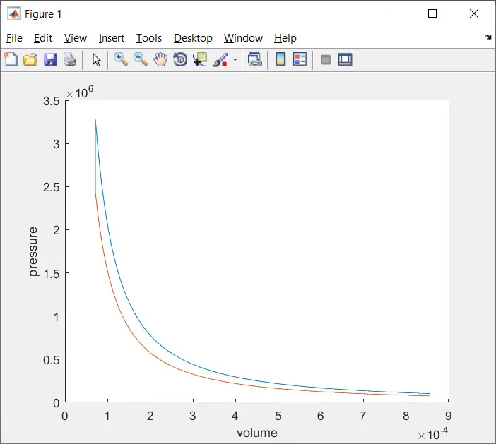
• Here the constant volume is correct.
• But the Compression Ratio & Expansion Ratio are represented by wrong path curves.
• In order to solve these issues, we need to use Thermodynamic relation during compression & Piston Kinematics to determine the change in volume at TDC & BDC

Piston Kinematics Equation Explanation:-

• Movement of Pistion from TDC to BDC & understanding how the combustion volume is changing as a function of a crank angle.

• Code is given as per the formula and values are assumed considering the code that is generated firstly.

Creating Function Template code:-

function [V] = Piston_kinematics_otto(bore,stroke,con_rod,cr,start_crank,end_crank)

a = stroke/2
R = con_rod/a

v_s = pi/4*bore^2*stroke;
v_c = v_s/(cr-1);
theta = linspace(start_crank,end_crank,100);

term1 = 0.5*(cr - 1);
term2 = R + 1 - cosd(theta);
term3 = (R^2 - sind(theta).^2).^0.5;

V = (1 +term1*(term2 - term3)).*v_c

end

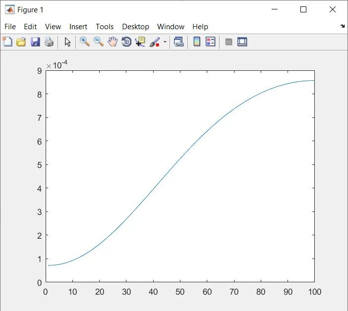
V_compression Plotting for the above code from command window:-

• V_compression = Piston_kinematics_otto(0.1,0.1,0.15,12,0,180)
• plot(V_compression)

Actual Code for Otto Cycle:-

%inputs 
gamma = 1.4
t3 = 1000

%state variables
p1 = 101325
t1 = 500

%Engine geometric parameters
bore = 0.1;
stroke = 0.1;
con_rod = 0.15;
cr = 12;

% calculating the swept volume and the clearance volume
v_swept = (pi/4)*bore^2*stroke;
v_clearance = v_swept/(cr-1);

v1 = v_swept + v_clearance
v2 = v_clearance

% state variables at state point 2 
%p2v2^gamma = p1v1^gamma
%p2 = p1*(v1/v2)^gamma = p1*cr^gamma

p2 = p1*cr^gamma;
constant_c = p1*v1^gamma;

 V_compression = Piston_kinematics_otto(bore, stroke, con_rod, cr, 180,0);

 P_compression = constant_c./V_compression.^gamma;
 
%p1v1/t1 = p2v2/t2   | t2 = p2*v2*t1/(p1*v1)
t2 = p2*v2*t1/(p1*v1);

%state variables at state point 3
v3 = v2

%p3v3/t3 = p2v2/t2 | p3 = p2*t3/t2
 p3 = p2*t3/t2
 
 constant_c = p3*v3^gamma;

 V_expansion= Piston_kinematics_otto(bore, stroke, con_rod, cr, 0,180);

 P_expansion = constant_c./V_expansion.^gamma;
 
 %state variables at state point 4
 v4 = v1
 
 %p3v3^gamma = p4v4^gamma | p4 = p3(v3/v4)^gamma
 p4 = p3*(v3/v4)^gamma

 % plotting
  hold on
 
 
plot( V_compression, P_compression)  
plot( V_expansion, P_expansion)

plot([v2 v3], [p2 p3], 'color', 'g')
plot([v4 v1], [p4 p1], 'color', 'b')
    
  
xlabel('volume')
ylabel('pressure')

% To calculate the thermal efficiency 
Thermal_efficiency = 1-(1/cr^(gamma-1))

Figure:-

To find the Thermal Efficiency:-

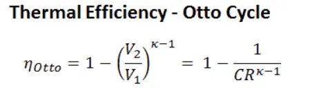
• Thermal_efficiency = 1-(1/cr^(gamma-1))

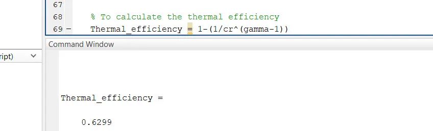
• Therefore 0.6299*100 = 62.99%
• The Approx Thermal Efficiency of Otto Cycle is ~63%

Google Drive Link:- https://drive.google.com/drive/folders/1wVEQo7GPjy7PFUmjqJEW8XXJGqJ5O0yl?usp=sharing