Linear convection II

Aim :

To find the numerical solution to the one-dimensional Linear Convection equation.

Objectives:

• For the particular value of C and time, the final velocity profiles should be analysed.
• The comparision should be made for various time step values, dt.
• To analyse the optimum or correct time step value.

Inputs:

• Domain length, L = 1m.
• Constant Velocity, C = 1.
• Number of grid points, n=80.
• The initial velocity is a step function. It is equal to 2m/s between x= 0.1 and 0.3 and 1m/s everywhere else.
• First-order forward differencing for the time derivative.
• First-order backward/rearward differencing for the space term.
• Time step is varied with the different values of 1e-4, 1e-3, 1e-2, and 1e-1.

Linear convection:

The one dimensional linear convection equation is represent below,

`(delu)/(delt)+C*(delu)/(delx)=0`

On the above equation, `(delu)/(delt)` term is referred as time derivative term. The first order forward differencing is applied for the time derivative term. By applying the forward differencing,

`(delu)/(delt)=(u(i)^(n+1)-u(i)^(n))/(Deltat)`

On the above equation, `(delu)/(delx)`term is reffered as the sapce term. The first order backward/rearward differencing is applied for the space derivative term. By applying the backward/rearward differencing,

`(delu)/(delx)=(u(i)^n-u(i-1)^n)/(Deltax)`

The next position of the velocity as a result of time marching can be obtained as,

`u(i)^(n+1)=u(i)^n-C*(Deltat)/(Deltax)*(u(i)^n-u(i-1)^n)`

By substituting the values of C, number of grid points and other values, the linear convection for various time step values are obtained.

MATLAB Code:

clear all
close all
clc

%Initializing the inputs

%Length of the domain
l=1;

%Constant velocity C
C=1;

%Total time and time step
t=0.4;
for dt=[1e-4,1e-3,1e-2,1e-1]

%Grid points
 n=80;

%Node points
 x=linspace(0,l,n);
 dx=x(2)-x(1);

%Starting and ending point where the velocity u is maximum at x coordinate
 x_start = 0.1;
 x_end = 0.3;

%Starting and ending point where the velocity is maximum for different grid
% points at x coordinate
 n_start = (x_start/dx)+1;
 n_end = (x_end/dx)+1;

%Initializing array and apply boundary condition
 u = ones(1,n);
 u(n_start:n_end)=2;

 u_old = u;
 u_initial = u;

%Time step
 nt = 0.4/dt;

%Time step loop
  for k = 1:nt
    
    %space loop
    for i=2:n
        u(i) = u_old(i)-(C*(dt/dx)*(u_old(i)-u_old(i-1)));
    end
    
    %updating the velocity
    u_old = u;
  end
    
    %Plotting
    figure(1)
    plot(x,u);
    axis([0 1 0 2.5])
    xlabel('Length')
    ylabel('Velocity')
    title('Velocity profile at different "dt" value')
    hold on
end
figure(1)
plot(x,u_initial,'k')
legend('dt=1e-4','dt=1e-3','dt=1e-2','dt=1e-1','Initial profile')

Code explanation:

• Initially, the length of the domain is assigned along with constant velocity C value.
• The number of grid points, time and time step values are assigned.
• The time step is assigned in a for loop for different values of dt = [1e-4,1e-3,1e-2,1e-1]
• The grid nodes are assigned and the stensil is found.
• Since the velocity changed for particular length value, the start and end point at the grid on which the velocity is maximum is found.
• Time step value is initialized.
• The time marching loop is opened.
• The space loop is opened in which the next velocity of the next time step is found by solving the final equation.
• The velocity is updated after solving the equation.
• Finally, the plotting is made to visualize the velocity profile at different time step dt values.

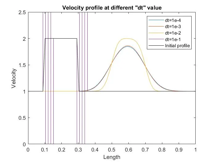
Output plots:

Conclusion:

• The velocity profile drops down can be visible in the result plot for various dt values. This is due to the artificial diffusion phenomenon. It is also known as numerical diffusion.
• The numerical diffusion is more at the dt=1e-4.
• The numerical diffusion phenomenon decreases by decreasing the value of dt and at the optimum dt value, the false diffusion phenomenon disappears.
• At dt=1e-1, there are distortion occurs at the velocity profile. This is because of gibbs phenomenon. The gibbs phenomenon tells that the result is unstable.
• Thus, the result plot concludes that the selection of optimum differencing scheme and time step dt value make the solution stable.