Linear convection I

Aim :

To find the numerical solution to the one-dimensional Linear Convection equation.

Objectives:

• For the particular value of C and time, the original and final velocity profiles should be analysed.
• The comparision should be made for various grid points, n.
• To analyse the optimum or correct grid point.

Inputs:

• Domain length, L = 1m.
• Constant Velocity, C = 1.
• Set time step = 0.01.
• The initial velocity is a step function. It is equal to 2m/s between x= 0.1 and 0.3 and 1m/s everywhere else.
• First-order forward differencing for the time derivative.
• First-order backward/rearward differencing for the space term.
• Time step and number of grid points should be variables in your calculation.

Linear convection:

The one dimensional linear convection equation is represent below,

`(delu)/(delt)+C*(delu)/(delx)=0`

On the above equation, `(delu)/(delt)` term is referred as time derivative term. The first order forward differencing is applied for the time derivative term. By applying the forward differencing,

`(delu)/(delt)=(u(i)^(n+1)-u(i)^(n))/(Deltat)`

On the above equation, `(delu)/(delx)`term is reffered as the sapce term. The first order backward/rearward differencing is applied for the space derivative term. By applying the backward/rearward differencing,

`(delu)/(delx)=(u(i)^n-u(i-1)^n)/(Deltax)`

The next position of the velocity as a result of time marching can be obtained as,

`u(i)^(n+1)=u(i)^n-C*(Deltat)/(Deltax)*(u(i)^n-u(i-1)^n)`

By substituting the values of C, time step and other values, the linear convection for various grid points are obtained.

MATLAB Code:

clear all
close all
clc

%Initializing the inputs

%Length of the domain
l=1;

%Constant velocity C
C=1;

%Total time and time step
t=0.4;
dt=0.01;

%Grid points
n=20;

%Node points
x=linspace(0,l,n);
dx=x(2)-x(1);

%Starting and ending point where the velocity u is maximum at x coordinate
x_start = 0.1;
x_end = 0.3;

%Starting and ending point where the velocity is maximum for different grid
% points at x coordinate
n_start = (x_start/dx)+1;
n_end = (x_end/dx)+1;

%Initializing array and apply boundary condition
u = ones(1,n);
u(n_start:n_end)=2;

u_old = u;
u_initial = u;

%Time step
nt = t/dt;

%Time step loop
for k = 1:nt
    
    %space loop
    for i=2:n
        u(i) = u_old(i)-(C*(dt/dx)*(u_old(i)-u_old(i-1)));
    end
    
    %updating the velocity
    u_old = u;
    
    %Plotting
    plot(x,u,'r');
    hold on
    plot(x,u_initial,'b');
    pause(0.3)
    axis([0 1 0 2.5])
    xlabel('Length')
    ylabel('Velocity')
    title('Velocity profile at each time step')
    legend('Velocity profile at various time step','Initial Velocity profile') 
end
    
    

Code explanation:

• Initially, the length of the domain is assigned along with constant velocity C value.
• The number of grid points, time and time step values are assigned.
• The grid nodes are assigned and the stensil is found.
• Since the velocity changed for particular length value, the start and end point at the grid on which the velocity is maximum is found.
• Time step value is initialized.
• The time marching loop is opened.
• The space loop is opened in which the next velocity of the next time step is found by solving the final equation.
• The velocity is updated after solving the equation.
• Finally, the plotting is made to visualize the velocity profile at various time step.

Output plots:

The velocity profile at various time step for different number of nodes value are shown below,

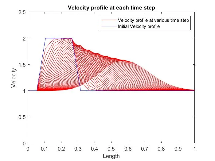
a) Velocity profile at number of nodes, n=20:

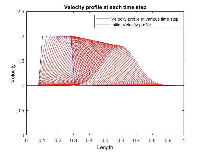
b) Velocity profile at number of nodes, n=40:

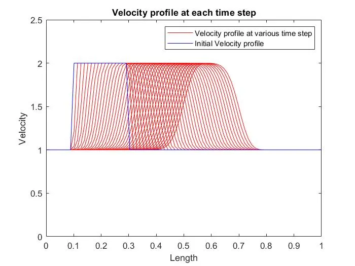
c) Velocity profile at number of nodes, n=80:

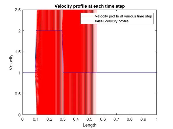
d) Velocity profile at number of nodes, n=160:

Conclusion:

• The velocity profile drops down can be visible in the result plot at n=20 and n=40. This is due to the artificial diffusion phenomenon. It is also known as numerical diffusion.
• The numerical diffusion is more at the number of node n=20.
• The numerical diffusion phenomenon decreases by increasing the number of nodes and at the optimum number of nodes value, the false diffusion phenomenon disappears.
• At the number of node n=80, the numerical diffusion phenomenon disappears, which tells that the number of node value 80 is the optimum or the best one.
• At n=160, there is a distortion on the plot. This is due to the gibbs phenomenon. The gibbs phenomenon tells that the result is unstable.
• Thus, the conclusion is that the selection of optimum differencing scheme and number of nodes value play a vital role in solving the problem to get the stable result.