Lateral Brush Tire Model

AIM: To plot the lateral brush tire model.

GIVEN DATA:

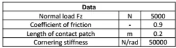
OBJECTIVE: To show the variation of lateral force and aligning moment with slip angle (0 to 15 deg).

GOVERNING EQUATION: The lateral brush tire model is conceptualized in the following three zones;

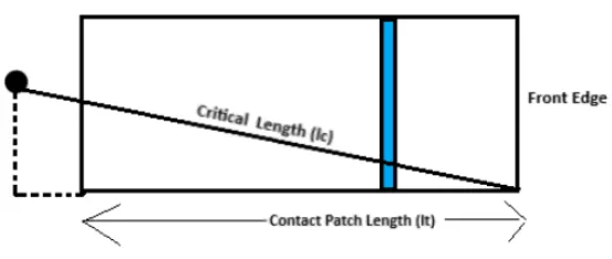
1. Adhesion region: Lateral force, `F_y = C_(alpha) .alpha` Aligning moment, `M_z = frac(C_(alpha) . l_t . alpha)(6)` where; `C_(alpha) = 1/2 . k_y . l_t^2` = Cornering stiffness (N/rad) `alpha` = Slip angle (degrees) `k_y` = stiffness (N/m^2) `l_t` = Length of contact patch (m)

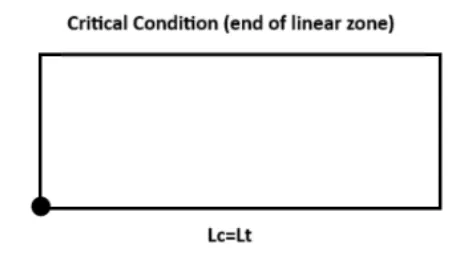
2. Critical point: Critical length, `l_c = frac(mu_p . F_z)(k_y . l_t . tan(alpha))` Critical slip angle, `alpha_c = frac(mu_p . F_z)(2 . C_a)` where; `mu_p` = Peak road-tire friction coefficient `F_z` = Normal load (N)

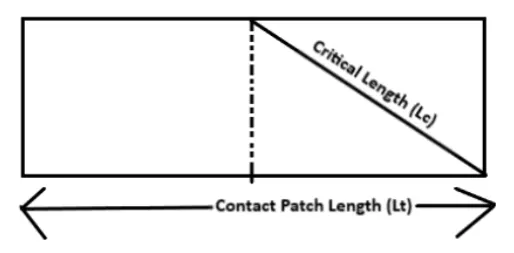
3. Sliding (Large Excitation) region: Lateral force, `F_y = mu_p . F_z - frac((mu_p . F_z)^2)(4.C_(alpha).tan(alpha))` Aligning moment, `M_z = frac((mu_p . F_z^2))(12.l_t.k_y.tan(alpha)) . [3 - frac(2.mu_p.F_z)(l_t^2.k_y.tan(alpha))]`

THEORY:

Lateral Force:

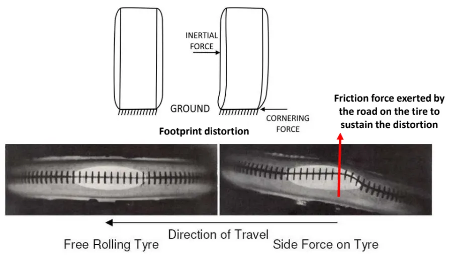
• Cornering force is applied (and this leads to the inertial force)
• The forces cause footprint distortion
• The rolling tread elements are deflected sideways
• Friction is what sustains this distortion and leads to the build-up of lateral force/shear stress
• Due to the distortion, the wheel travels in a different direction from where it points

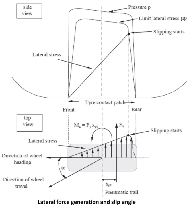
When a rolling pneumatic tire is subjected to a lateral force, an angle called slip angle is created between the direction of tire heading and the direction of travel. When a tire rolls at a slip angle, the tread elements that come into contact with the road are deflected sideways due to, causing a lateral stress buildup. When the lateral stress exceeds the boundary set by friction limits, sliding occurs and the lateral stress follows the boundary limit distribution. The area of the stress buildup is a measure of the resulting cornering force Fy. As the shape of the stress distribution is approximately triangular, the lateral force acts through the centroid. The distance between this centroid and the wheel centerline is called the pneumatic trail. This mechanism is not instantaneous as the lateral force generation lags the slip angle by a certain distance that the tire has to roll called relaxation length. During high-speed driving, this may be interpreted as sluggishness in turn-in.

SOLUTION:

Programming Language: MATLAB

Code:

% Lateral Brush Tire Model

% Input data:

F_z = 5000;   % Normal force (N)
mu = 0.9;     % Peak road-tire friction coefficient
l_t = 0.2;    % Length of tire contact patch (Assumed)
C_a = 50000;  % Lateral stiffness (N)


% Solution:

k_y = 2*C_a/(l_t^2);
alpha_c = mu*F_z/(2*C_a);   % Critical slip

for i=1:300
    alpha(i) = (i-1)*0.1*pi/180;
    
    if alpha(i) < alpha_c   % Adhesion region
        F_y(i) = C_a*alpha(i);
        M_z(i) = C_a*l_t*alpha(i)/6;
        
    else                    % Slipping region
        F_y(i) = mu*F_z - (mu*F_z)^2 / (4*C_a*tan(alpha(i)));
        M_z(i) = ((mu*F_z)^2 / (12*l_t*k_y*tan(alpha(i)))*(3 - 2*mu*F_z / (l_t^2*k_y*tan(alpha(i)))));
    end
end


% Plot:

subplot(2,1,1)
plot(alpha*180/pi, F_y,'linewidth',3)
xlabel('Slip angle (degrees)')
ylabel('Lateral force (N)')
title('Lateral force vs Slip angle')
grid on
hold on

subplot(2,1,2)
plot(alpha*180/pi, M_z,'linewidth',3)
xlabel('Slip angle (degrees)')
ylabel('Aligning moment (Nm)')
title('Aligning moment vs Slip angle')
grid on
hold on

------------------------------------------------------------------------------------------------------

% Reduced Friction Case

% Input data:

F_z = 5000;   % Normal force (N)
mu = 0.6;     % Peak road-tire friction coefficient
l_t = 0.2;    % Length of tire contact patch (Assumed)
C_a = 50000;  % Lateral stiffness (N)


% Solution:

k_y = 2*C_a/(l_t^2);
alpha_c = mu*F_z/(2*C_a);   % Critical slip

for i=1:300
    alpha(i) = (i-1)*0.1*pi/180;
    
    if alpha(i) < alpha_c   % Adhesion region
        F_y(i) = C_a*alpha(i);
        M_z(i) = C_a*l_t*alpha(i)/6;
        
    else                    % Slipping region
        F_y(i) = mu*F_z - (mu*F_z)^2 / (4*C_a*tan(alpha(i)));
        M_z(i) = ((mu*F_z)^2 / (12*l_t*k_y*tan(alpha(i)))*(3 - 2*mu*F_z / (l_t^2*k_y*tan(alpha(i)))));
    end
end


% Plot:

subplot(2,1,1)
plot(alpha*180/pi, F_y,'linewidth',3)
xlabel('Slip angle (degrees)')
ylabel('Lateral force (N)')
title('Lateral force vs Slip angle')
legend('mu = 0.8','mu = 0.6')
grid on
hold on

subplot(2,1,2)
plot(alpha*180/pi, M_z,'linewidth',3)
xlabel('Slip angle (degrees)')
ylabel('Aligning moment (Nm)')
title('Aligning moment vs Slip angle')
legend('mu = 0.8','mu = 0.6')
grid on

Output:

Plot:

CONCLUSION:

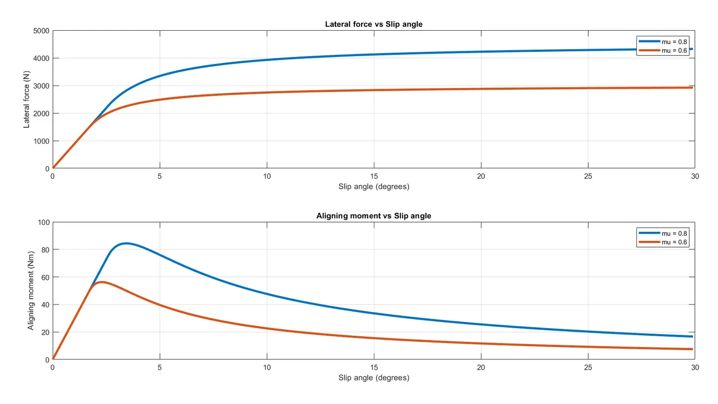
From the above results, we can infer that by reducing the coefficient of friction, the cornering force and aligning moment decreases significantly within the tire. Also, the peak lateral force is less than the normal load that is imposed on the tire.

- Adhesion region: The peak occurs early in the reduced friction case as compared to the normal one, thus indicating the ability of tire to be within the adhesion zone.

- Critical point: The peak in traction force and aligning moment is more in case of higher frictional coefficient and it occurs at higher slip angle.

- Sliding region: Beyond the peak value, the lateral force decreases and aligning moment converges beyond that point.