How to solve an Otto cycle using Matlab

AIM

To write a code that can solve otto cycle and make plots for it.

OBJECTIVE

A program to create P-V diagram for an otto cycle and to calculate its thermal efficiency

THEORY

An Otto cycle is an idealized thermodynamic cycle that describes the functioning of a typical spark ignition piston engine. It is the thermodynamic cycle most commonly found in automobile engines.

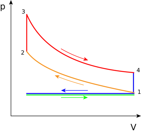
It consists of 4 major processes:

Process 1 to 2: During this phase the piston will be drawn up, so it can compress the fuel-air mixture that entered the chamber. The compression causes the mixture to increase slightly in pressure and temperature—however, no heat is exchanged. In terms of thermodynamics, this is referred to as an adiabatic process. When the cycle reaches point 2, that is when the fuel is met by the spark plug to be ignited.

Process 2 to 3: This is where combustion occurs due to the ignition of fuel by the spark plug. The combustion of the gas is complete at point 3, which results in a highly pressurized chamber that has a lot of heat (thermal energy). In terms of thermodynamics, this is referred to as an isochoric process.

Process 3 to 4: The thermal energy in the chamber as a result of combustion is used to do work on the piston—which pushes the piston down—increasing the volume of the chamber. This is also known as the power stroke because it is when the thermal energy is turned into motion to power the machine or vehicle.

Process 4 to 1 and exhaust phase: From process 4 to 1, all waste heat is expelled from the engine chamber. As the heat leaves the gas, the molecules lose kinetic energy causing the decrease in pressure. Then the exhaust phase occurs when the remaining mixture in the chamber is compressed by the piston to be "exhausted" out, without changing the pressure.

CODE

clear all
close all
clc

%inputs
gamma=1.4;
t3=2300;

%state variables
p1=101325;
t1=500;

%engine geometric parameters
bore=0.1;
stroke=0.1;
con_rod=0.15;
cr=12;

%calculating the swept volume and clearance volume
v_swept=(pi/4)*bore^2*stroke;
v_clearance=v_swept/(cr-1);

v1=v_swept+v_clearance;
v2=v_clearance;

%state variables at state point 2
%p2v2^gamma=p1v1^gamma
%p2 = p1*(v1/v2)^gamma = p1*cr^gamma
p2=p1*cr^gamma;

%p1v1/t1 = p2v2/t2 | t2=p2v2t1/(p1v1)
t2=p2*v2*t1/(p1*v1);

%using the function engine_kinematics
constant_c=p1*v1^gamma;
v_compression=engine_kinematics(bore,stroke,con_rod,cr,180,0);
p_compression=constant_c./v_compression.^gamma;

%state variables at state point 3
v3=v2;

%p3v3/t3 = p2v2/t2 | p3=p2t3/t2
p3=p2*t3/t2;

%again using the function engine_kinematics
constant_c=p3*v3^gamma;
v_expansion=engine_kinematics(bore,stroke,con_rod,cr,0,180);
p_expansion=constant_c./v_expansion.^gamma;

%state variables at state point 4
v4=v1;

%p3v3^gamma = p4v4^gamma | p4=p3(v3/v4)^gamma
p4=p3*(v3/v4)^gamma;

%to calculate the Thermal efficiency of an otto cycle
% Thermal efficiency = 1-(v2/v1)^(gamma-1) = 1-(1/cr^(gamma-1))

Thermal_efficiency=(1-(1/cr^(gamma-1)))*100

%plotting the PV diagram
figure(1)
hold on
plot(v_compression,p_compression,'color','r','linewidth',2)
plot([v2 v3],[p2 p3],'color','b','linewidth',2)
plot(v_expansion,p_expansion,'color','y','linewidth',2)
plot([v4 v1],[p4 p1],'color','black','linewidth',2)
title('P-V Diagram of otto cycle')
xlabel('Volume')
ylabel('Pressure')
legend('Isentropic compression','CV heat addition','Isentropic expansion','CV heat rejection')

EXPLANATION

• Initially the basic inputs like engine geometric parameters and initial state variables are declared.
• The swept volume and clearance volume are calculated using compression ratio, bore and stroke values.
• The values at different state points are calculated using the various thermodynamic relations mentioned in the above code.
• Inorder to obtain the perfect curves for each isentropic compression and isentropic expansion, we need to intoduce a new function into this code named as 'engine_kinematics', which is mentioned below

• function[V]=engine_kinematics(bore,stroke,con_rod,cr,start_crank,end_crank)
  
  a=stroke/2;
  R=con_rod/a;
  
  v_s=pi/4*bore^2*stroke;
  v_c=v_s/(cr-1);
  
  theta=linspace(start_crank,end_crank,100);
  
  term1=0.5*(cr-1);
  term2=R+1-cosd(theta);
  term3=(R^2-sind(theta).^2).^0.5;
  
  V=(1+term1*(term2-term3)).*v_c;
  end
  

• This function uses the equation of volume trace for each compression and parameters given
• To plot the curves we use the output from the function and join it with the other state variables for pressure and volume at each stages during the process.
• The Thermal efficiency of the otto cycle is obtained from the relation:-
• 

RESULT

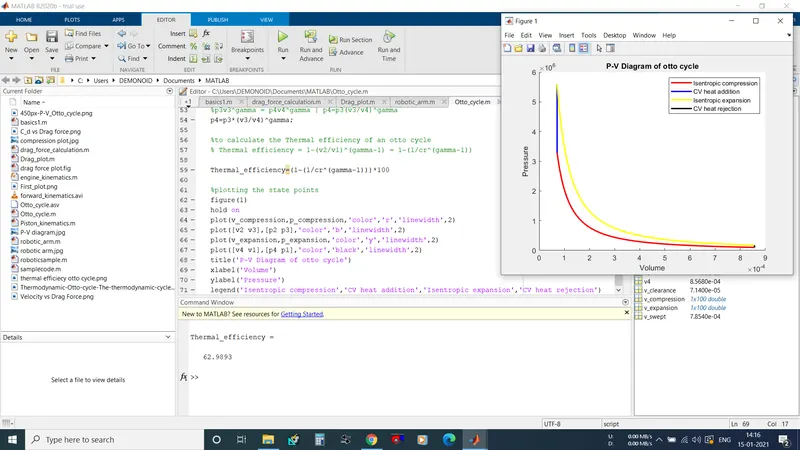
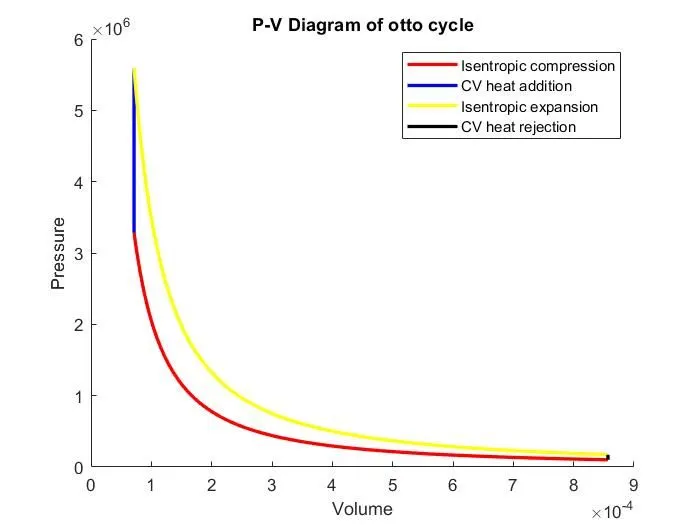
The thermal efficiency was obtained as 62.99%

PROBLEMS FACED DURING CODING

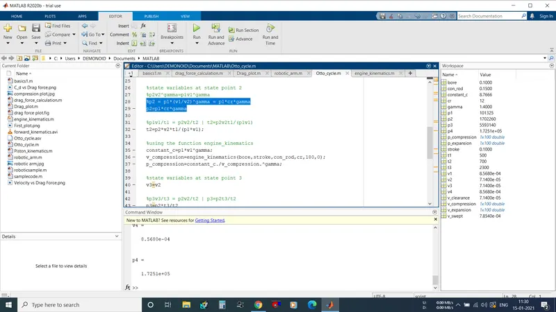
• There was a problem with having the wrong pressure and volume at state 2

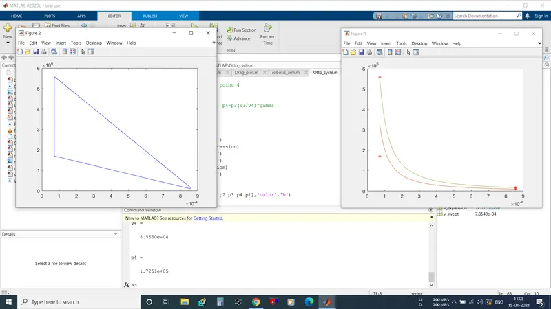
• The problem was resolve by finding an error in the calculation of p2, a wrong operator (*) was used intead of (^) to power the expression with gamma.

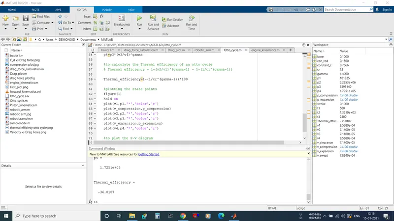
• While calculating the thermal efficiency, the value obtained was negative(-).
• Resolved by providing necessary brackets() wherever needed to correct the expression.

CONCLUSION

The Otto cycle is another example of a reversible cycle that only exists in theory. We study the Otto cycle to understand what takes place inside the internal combustion engine. In other words, for all assumption purposes, we can approximate the cycle taking place inside the internal combustion engine as the Otto cycle.

The program to solve an otto cycle and plot its P-V diagram and calculate it's Thermal efficiency was completed successfully and the results are provided.