Optimisation using Genetic Algorithm
AIM:
Writing a program in Matlab to find the global maxima of a function using Genetic algorithm.
THEORY:
A genetic algorithm is a search heuristic that is inspired by Charles Darwin's theory of natural evolution. This algorithm reflects the process of natural selection where the fittest individuals are selected for reproduction in order to produce offspring of the next generation.
Genetic algorithms are commonly used to generate high-quality solutions to optimization and search problems by relying on biologically inspired operators such as mutation, crossover and selection.
UNDERSTANDING THE SYNTAX OF GA:
x = ga(fun,nvars) finds a local unconstrained minimum, x, to the objective function, fun. nvars is the dimension (number of design variables) of fun.
x = ga(fun,nvars,A,b) finds a local minimum x to fun, subject to the linear inequalities A*x ≤ b. ga evaluates the matrix product A*x as if x is transposed (A*x').
x = ga(fun,nvars,A,b,Aeq,beq) finds a local minimum x to fun, subject to the linear equalities Aeq*x = beq and A*x ≤ b. (Set A=[] and b=[] if no linear inequalities exist.) ga evaluates the matrix product Aeq*x as if x is transposed (Aeq*x').
x = ga(fun,nvars,A,b,Aeq,beq,lb,ub) defines a set of lower and upper bounds on the design variables, x, so that a solution is found in the range lb ≤ x ≤ ub. (Set Aeq=[] and beq=[] if no linear equalities exist.)
x = ga(fun,nvars,A,b,Aeq,beq,lb,ub,nonlcon) subjects the minimization to the constraints defined in nonlcon. The function nonlcon accepts x and returns vectors C and Ceq, representing the nonlinear inequalities and equalities respectively. ga minimizes the fun such that C(x) ≤ 0 and Ceq(x) = 0. (Set lb=[] and ub=[] if no bounds exist.)
x = ga(fun,nvars,A,b,Aeq,beq,lb,ub,nonlcon,options) minimizes with the default optimization parameters replaced by values in options. (Set nonlcon=[] if no nonlinear constraints exist.) Create options using optimoptions.
x = ga(fun,nvars,A,b,[],[],lb,ub,nonlcon,IntCon) or x = ga(fun,nvars,A,b,[],[],lb,ub,nonlcon,IntCon,options) requires that the variables listed in IntCon take integer values.
x = ga(problem) finds the minimum for problem, where problem is a structure.
[x,fval] = ga(___), for any previous input arguments, also returns fval, the value of the fitness function at x.
[x,fval,exitflag,output] = ga(___) also returns exitflag, an integer identifying the reason the algorithm terminated, and output, a structure that contains output from each generation and other information about the performance of the algorithm.
[x,fval,exitflag,output,population,scores] = ga(___) also returns a matrix population, whose rows are the final population, and a vector scores, the scores of the final population.
FORMULA:
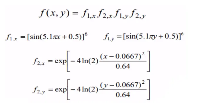
All the above-mentioned formulae are used for writing a program for stalagmite function which is then optimised using GA to find the global maximum. These are used for writing a code in Matlab.
MATLAB PROGRAMME:
Main function:
x=linspace(0,0.6,150);
y=linspace(0,0.6,150);

[xx,yy]=meshgrid(x,y);
number_of_cases=50

for i=1:length(xx)
    for j=1:length(yy)
        input_vector(1)=xx(i,j);
        input_vector(2)=yy(i,j);
        f(i,j)=stalagmite(input_vector);
    end
end

figure(1)
surfc(xx,yy,-f);
xlabel('x-value');
ylabel('y-value');
shading interp
[inputs,fval]=ga(@stalagmite,2)

%study-1 STATISTICAL BEHAVIOUR
tic
for i=1:number_of_cases
    [inputs,fopt(i)]=ga(@stalagmite,2);
    xopt(i)=inputs(1);
    yopt(i)=inputs(2);
end
study1_time=toc

figure(2)
subplot(2,1,1);
hold on
surfc(x,y,-f);
shading interp
plot3(xopt,yopt,-fopt,'marker','o','markersize',5,'markerfacecolor','r');
title('Unbounded inputs');
subplot(2,1,2);
plot(-fopt);
xlabel('No. of iterations');
ylabel('Function maximum value');

%study-2 STATISTICAL BEHAVIOUR with Lower and Upper bounds
tic
for i=1:number_of_cases
    [inputs,fopt(i)]=ga(@stalagmite,2,[],[],[],[],[0;0],[0.6;0.6]);
    xopt(i)=inputs(1);
    yopt(i)=inputs(2);
end
study2_time=toc

figure(3)
subplot(2,1,1);
hold on
surfc(x,y,-f);
shading interp
plot3(xopt,yopt,-fopt,'marker','o','markersize',5,'markerfacecolor','r');
title('Bounded inputs');
subplot(2,1,2);
plot(-fopt);
xlabel('No. of iterations');
ylabel('Function maximum value');

%study-3 Increasing GA populationsize
options=optimoptions('ga')
options=optimoptions(options,'PopulationSize',300)

tic
for i=1:number_of_cases
    [inputs,fopt(i)]=ga(@stalagmite,2,[],[],[],[],[0;0],[0.6;0.6],[],[],options);
    xopt(i)=inputs(1);
    yopt(i)=inputs(2);
end
study3_time=toc

figure(4)
subplot(2,1,1);
hold on
surfc(x,y,-f);
shading interp
plot3(xopt,yopt,-fopt,'marker','o','markersize',5,'markerfacecolor','r');
title('Bounded inputs with population size');
subplot(2,1,2);
plot(-fopt);
xlabel('No. of iterations');
ylabel('Function maximum value');
Side function:
function f=stalagmite(input_vector)

X=input_vector(1);
Y=input_vector(2);

f1=[sin(5.1*pi*X+0.5)]^6;
f2=[sin(5.1*pi*Y+0.5)]^6;
f3=exp(-4*log(2)*(X-0.0667)^2/0.64);
f4=exp(-4*log(2)*(Y-0.0667)^2/0.64);

f=-f1*f2*f3*f4;
end
The side function here is basically a stalagmite function which is used or called in the main function for finding its global maxima.
RESULTS:
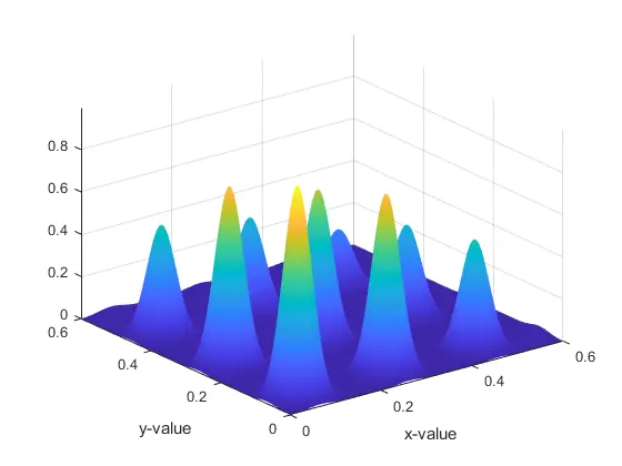
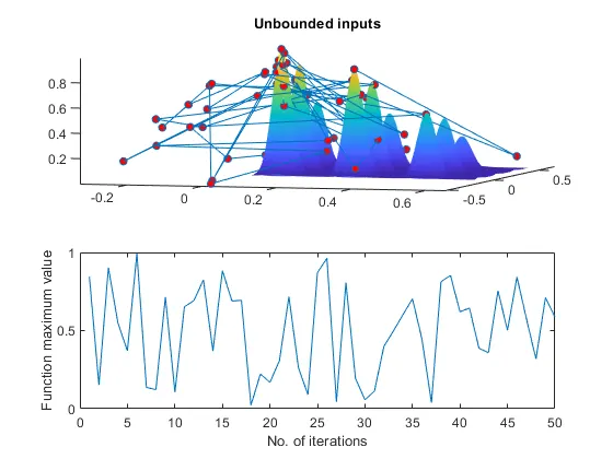
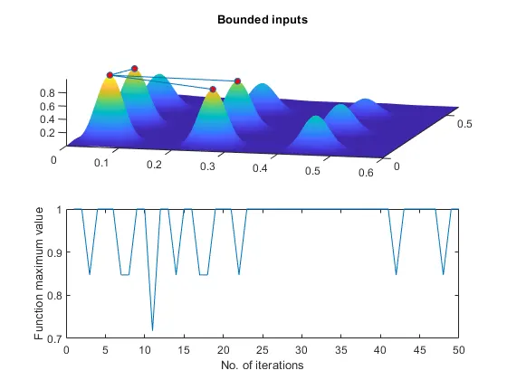
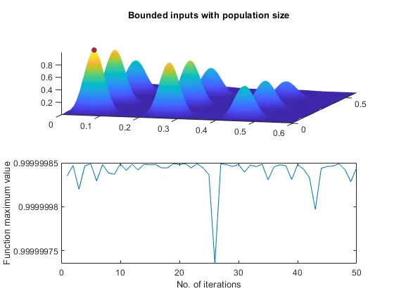
The plots for function maximum vs no. of iterations is shown below
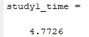
Study time results:
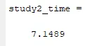
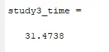
DISCUSSION OF RESULTS/CONCLUSION:
In case study 1, 2 and 3 the genetic algorithm performs differently. With no additional boundary conditions, the values of global maximum try to change in each case as the genetic algorithm randomly picks values and uses them to find the global maximum. By giving the upper and lower boundary limits the values of x and y are restricted within that range and thus making it easier for taking sets of values to find global maxima in this case. If we see case 3 then there’ll be additional input given which is population size. This increases the data points and helps to converge to a solution quickly. In case 2 there are 4 points in between which the global maximum is and in case 3 there’s exactly one point being found out which is the global maxima. We can even see the study time’s in all the cases. As the input conditions are increasing then the time to evaluate the results is also increasing. Thus, by using the above code the global maxima of the stalagmite function is achieved.
ERRORS:
No errors were seen during the entire program.
BIBLIOGRAPHY: