Parametric study on a Gate valve using Ansys Fluent
Aim – Three dimensional parametric study on a gate valve using Ansys Fluent.
Introduction –
Gate valves work by inserting a rectangular gate or wedge into the path of a flowing fluid. They are operated by a threaded stem which connects the actuator (generally a hand wheel or motor) to the stem of the gate. If the valve has a rising stem its position can be seen just by looking at the position of the stem. When fully open, a gate valve has no obstruction in the flow path and so has a very low pressure drop. If the fluid is very viscous a special type of gate valve known as a knife gate valve can be used.
One reason that gate valves are not normally used to regulate flow is that the flow rate of the fluid is not proportional to the amount that the valve is open. Moreover, a partially open gate valve may suffer from vibration in which the valve may move from its assigned position. Also the gate and seat may be subject to excessive wear if the valve is partially open.
In the present study, the partial opening effect on a pressure drop across a gate valve and thus, flow rate has been studied using Ansys parametric study tool.
Modelling and Solving approach –
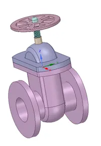
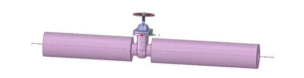
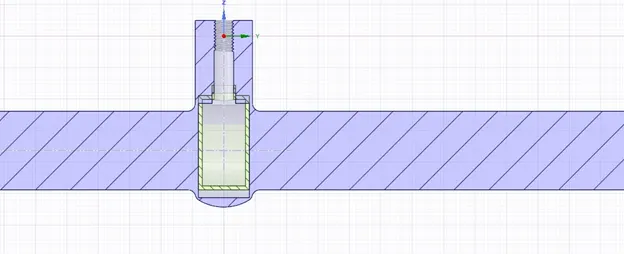
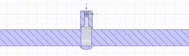
Solid Model – A 3D model of the gate valve was already provided. Since we need to perform only fluid flow study, thus all the parts of the solid model were suppressed. After this, the inlet and outlet surfaces of the gate valve body (part named as bottom) were pulled by 800 mm each using the Pull feature of Spaceclaim. All the other parts except the disc and spindle were hidden. The gate disc was the lifted up 10 mm using the move feature of Spaceclaim. The lift of the gate disc has been selected as the input parameter for each design point. Volume extraction feature (using edge selection) was then employed to extract the fluid volume by selecting the inlet outlet and edge below the bonnet of the gate valve body. The order of the above steps is important. If we move the gate valve disc after volume extraction then we also need to update the volume to accommodate the changes. To keep the volume updated during each of the study, the update as per context selection was made by right clicking on the volume subcomponent and selecting the option. The geometry was then exported to Ansys Mesher. The image of the model in Spaceclaim is provided below –
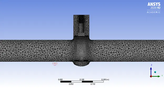
Meshing – Tetrahedral mesh has been utilized to mesh the 3D geometry with a global element size of 6 mm. High mesh count is necessary to prevent inaccuracies in high lift cases and also to ensure better convergence. Named selections are also created.
|
Method |
Tetrahedral |
|
Global Element size |
6 mm |
|
Capture curvature |
Yes |
|
Capture Proximity |
No |
|
Number of elements |
413511 |
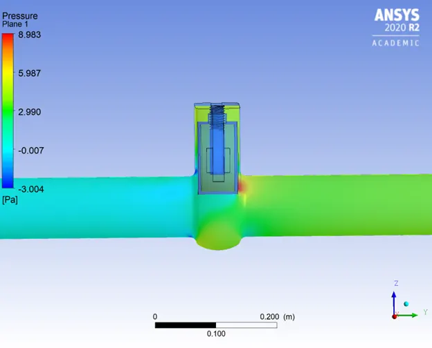
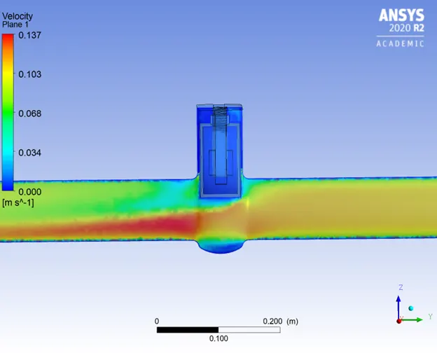
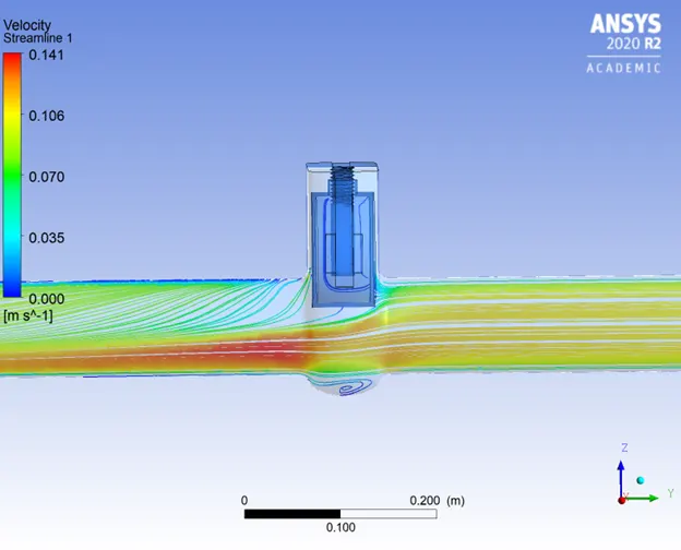
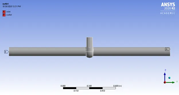
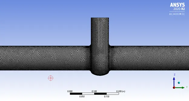
The images for 10 mm lift of gate disc has been shown below.
Solver Settings – Ansys Fluent was used as the solver and steady state simulations have been performed using a pressure based solver. Gravity was enabled in the negative y axis.
Boundary conditions and materials – Water was added in the materials and the cell zone conditions were then changed to accommodate water as the working fluid. To prevent any errors, air was deleted from the materials panel after this.
|
Named Selection |
Boundary condition (Value) |
|
Inlet |
Pressure Inlet (10 Pa gage) |
|
Outlet |
Pressure outlet (0 Pa gage) |
Computational model – To check if the flow is laminar or turbulent, we need to find the Reynolds number (And thus inlet velocity, which has not been defined). This can be done either by using Bernoulli’s equations or Ansys Fluent. We use the latter. If we chose standard initialization and compute from inlet we get the inlet velocity of 0.1415 m/s. The pipe diameter is 100 mm. Thus, Reynolds number is
`Re= (998.2*0.1415*0.1)/0.001003 ≈14082`
This lies in the turbulent region for internal flows. Thus, Realizable k-epsilon (scalable wall function) model has been used.
Spatial Discretization – Coupled Pressure velocity coupling scheme was used to solve the Navier Stokes Equations. The default solution controls and methods have been used.
|
Gradient |
Least Squares Cell Based |
|
Pressure |
Second Order |
|
Momentum |
Second Order Upwind |
|
Turbulent kinetic energy |
First order upwind |
|
Turbulent dissipation rate |
First order upwind |
The solution has been initialized using the Standard Initialization method (from inlet) and has been run for 250 iterations for each design point.
Results and Discussion –
A known limitation of Ansys Fluent is that it gets stuck at updating solution stage in a parametric study if either any graphics window is open in fluent. To avoid this, none of the plots (inlet and outlet mass flow, and residuals) have been plotted in fluent.
After the study is complete, the residual plots can be extracted. To check if convergence has been reached the files of outlet mass flow have been checked for convergence during the end of iterations.
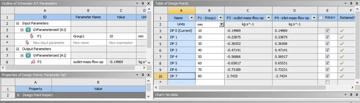
The negative sign indicates the mass outflow.
After a successful study, the table of design points should look like the below image. It is to be noted that in the below image DP7 results is not accurate, thus that particular design point was re simulated by modifying the mesh. Since the pipe diameter is 100 mm, thus the lift varies from 10 mm to 80 mm.
The measure of gate valve efficiency at allowing fluid flow can be related by two coefficients known as Flow coefficient (Cv) and Flow Factor (Kv). The relation for the both is same but the units are different. They are given as
`C_v=K_v= Q*√((SG of fluid)/(∆P))`
|
Q |
SG |
`DeltaP` | |
|
Kv |
m3/h |
1 (fluid = water) |
bars |
|
Cv |
Gallons per minute |
1 (fluid = water) |
psi |
The below table highlights the important results of this study.
| Opening % | Inlet Mass flow (kg/s) |
Outlet mass flow (kg/s) |
Inlet Avg Press (Pa) |
Outlet Avg Press (Pa) |
Pressure drop (Pa) |
Flow Rate (m3/h) |
Pressure drop (bars) |
Pressure drop (psi) |
Flow Coefficient,Cv |
Flow Factor Kv |
Kv/Cv |
| 10 (DP0) | 0.14957591 | -0.1495759 | 10 | 0.18526896 | 9.81473104 | 0.53847324 | 9.81473E-05 | 0.001423509 | 62.79668 | 54.35318 | 0.865542 |
| 20(DP1) | 0.23989142 | -0.23989077 | 10 | 0.4747418 | 9.5252582 | 0.86360677 | 9.52526E-05 | 0.001381524 | 102.2326 | 88.48663 | 0.865542 |
| 30(DP2) | 0.36508 | -0.36552 | 10 | 1.07839 | 8.92161 | 1.315872 | 8.92161E-05 | 0.001293972 | 160.9548 | 139.3131 | 0.865542 |
| 40(DP3) | 0.47610118 | -0.47608143 | 10 | 1.8760656 | 8.1239344 | 1.71389315 | 8.12393E-05 | 0.001178279 | 219.691 | 190.1518 | 0.865542 |
| 50(DP4) | 0.56642324 | -0.56618079 | 10 | 2.651714 | 7.348286 | 2.03825084 | 7.34829E-05 | 0.001065781 | 274.7112 | 237.7741 | 0.865542 |
| 60(DP5) | 0.67965437 | -0.67907014 | 10 | 3.7071952 | 6.2928048 | 2.4446525 | 6.2928E-05 | 0.000912696 | 356.0465 | 308.1733 | 0.865542 |
| 70(DP6) | 0.77321322 | -0.78006304 | 10 | 5.1585692 | 4.8414308 | 2.80822694 | 4.84143E-05 | 0.000702191 | 466.2911 | 403.5946 | 0.865542 |
| 80(DP7) | 0.83488801 | -0.77858706 | 10 | 5.0172127 | 4.9827873 | 2.80291342 | 4.98279E-05 | 0.000722694 | 458.7597 | 397.0759 | 0.865542 |
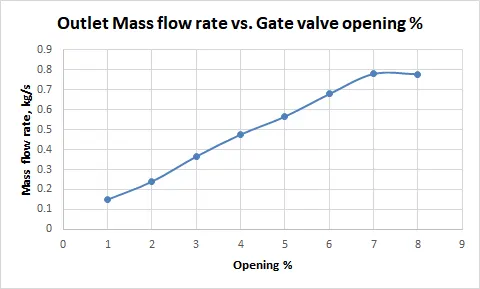
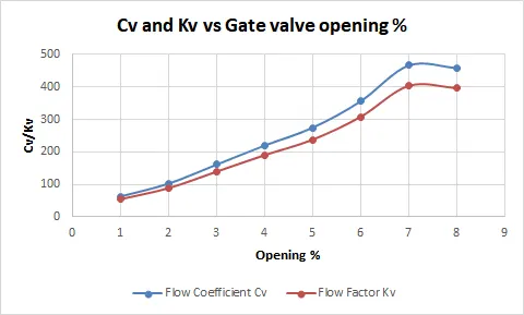
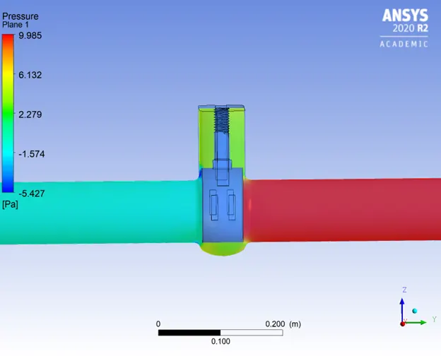
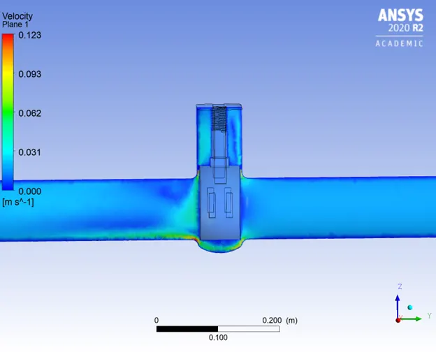
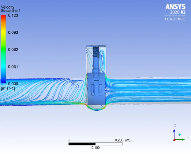
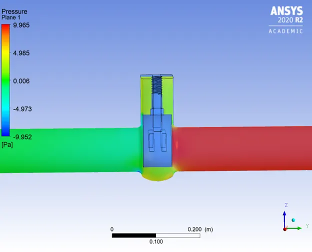
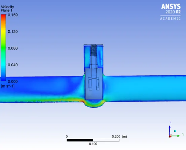
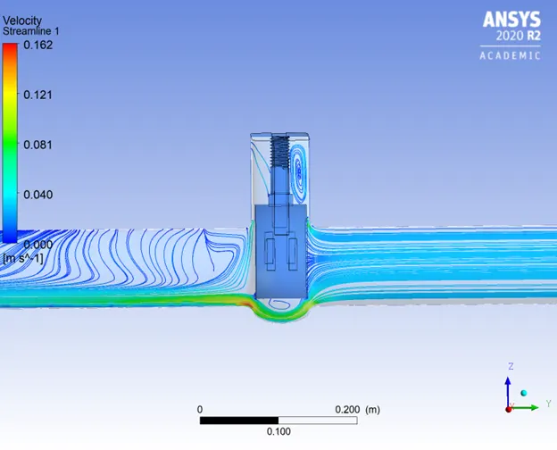
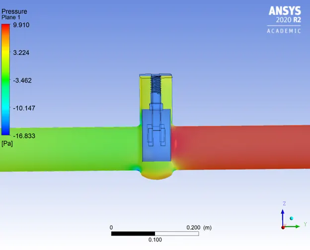
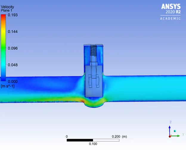
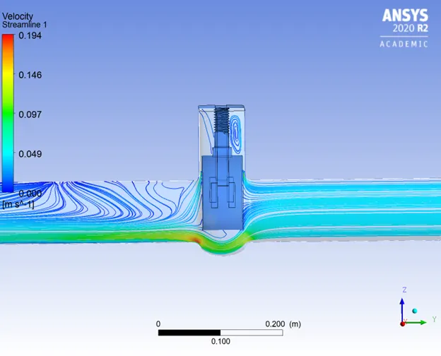
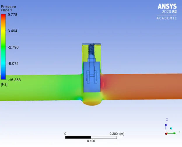
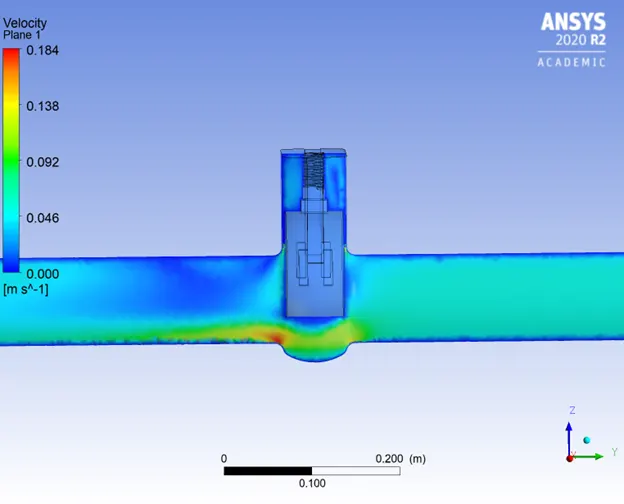
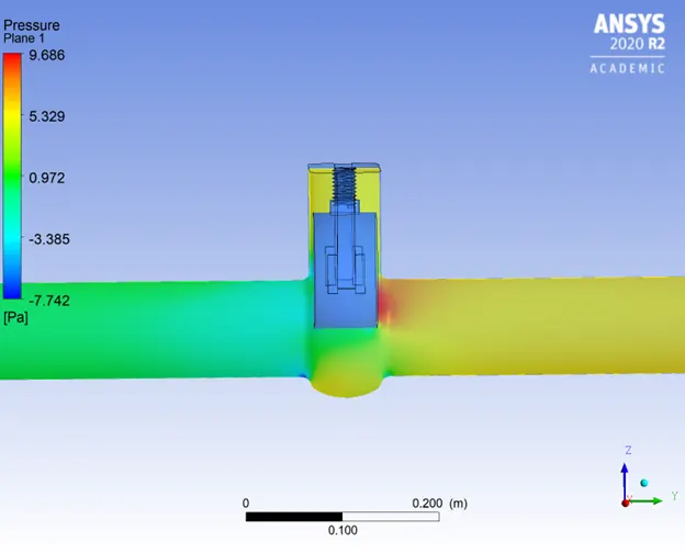
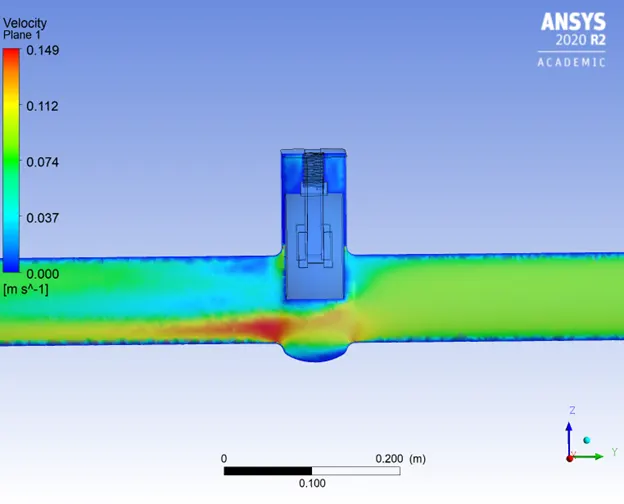
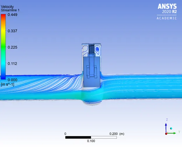
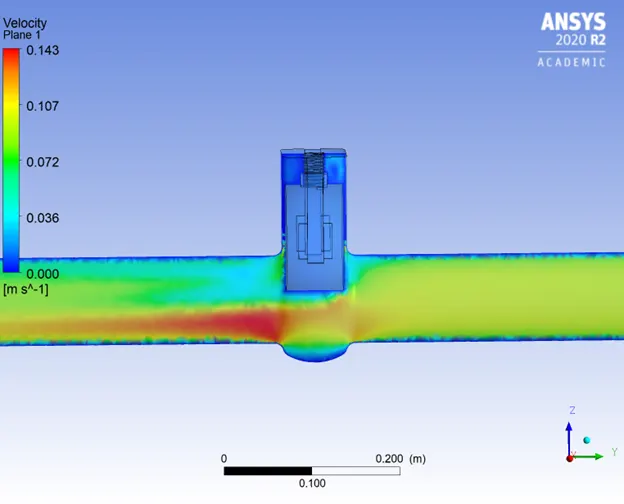
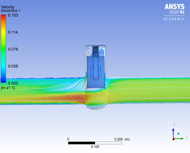
Some relevant contours of the study are attached herewith. The change in fluid volume can be clearly observed in each of the design point.
DP0
DP1
DP2
DP3
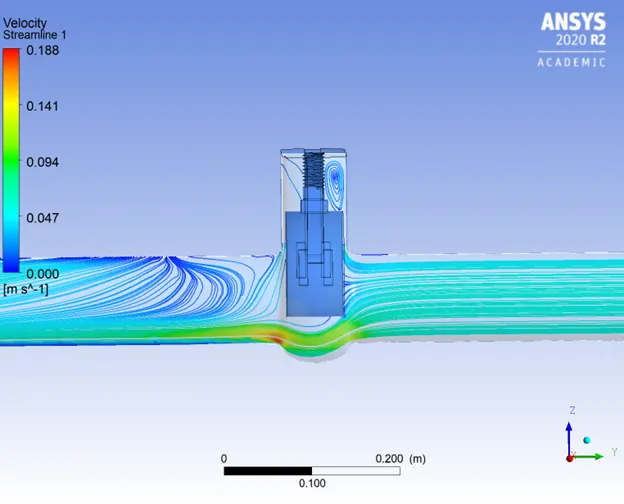
DP4
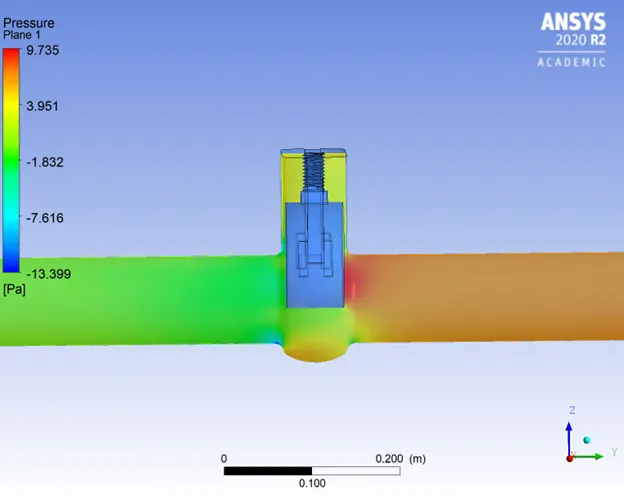
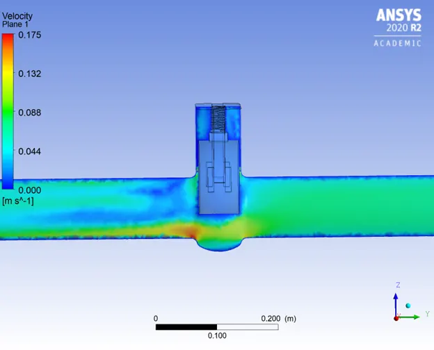
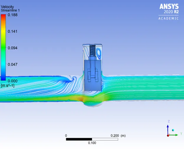
DP5
DP6
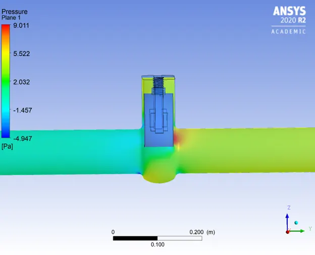
DP7