FVM Literature Review
Aim:
To made an extensive literative review on Finite Volume Method (FVM) used in computational fluid dynamics.
Introduction:
The prototype for a component or object can be analysed by various methods. The three methods are, a) Analytical method b) Numerical method and c) Experimental method. Numerical method is the best method when compared with other two methods. The numerical method is employed in the back end of computational mechanics. In numerical methods, there are various methods available for solving the unique problems. They are,
- Finite Element Method (FEM)
- Boundary Element Method (BEM)
- Finite Volume Method (FVM)
- Finite Difference Method (FDM)
Finite Element Method - The Finite element method is used in various structural, fluid flow, heat transfer and electromagnetic analysis. The FEM is a type of numerical method in which the governing equation in the form of partial differential equation is solved. To solve the equation, the component is divided into various small elements and the changes occur at each elements are analysed.
Boundary Element Method - The Boundary element method is a type of numerical method in which the linear partial differential equation is solved and it was formulated as boundary integral equations. This method is implemented to solve the various problems such as electromagnetics, fracture mechanics, contact mechanics and fluid mechanics problems. This method is implemented in the problem having small surface/volume ratio. It solves the problem by creating a mesh over the surface of the component.
Finite Volume Method - The finite volume method is one of the important numerical method which was applied in computational fluid dynamics(CFD) problems. In this method, the partial differential equations are evaluated into algebraic equations. Using divergence theorem, the volume integrals in the partial differential equations which containing divergence term and it is converted into surface integrals.
Finite Difference Method - The finite difference method is a numerical method in which the governing equation which was in the form of ordinary differential equation or partial differential equation is converted into a system of linear equations and then it is solved by matrix algebra techniques. The ODE or PDE is converted into a system of linear equations by applying different schemes, forward, backward and central differencing schemes.
Drawbacks of FDM:
The Finite Difference Method and the Finite Volume Method are the two methods which are used to solve the CFD problems. The finite difference method is used to solve the various 1D, 2D and some 3D CFD problems. Many 1D and 2D problems can be easily solved to get the converged results using FDM process. But the FDM has some drawbacks in solving some CFD problems. It increases the time to get the converged results and sometimes it failed to get the converged results. One of the major drawback of FDM is, to get the converged results, the mesh should be defined in particular with any one axis or any two axes. This become complicated for the 3D objects because it has 3 axes coordinates. They can also solved using FDM by applying variable tranformation approach. But it is too complicated one and it took huge time to get the converged results. Thus, the FDM is replaced with FVM to solve that complicated 3D objects.
Finite Volume Method:
Finite volume method is one in which the partial differential equations are evaluated into algebraic equations. Instead of analysing the results about a point in FDM, in FVM the results are analysed about a volume. The FVM is used by many CFD packages around the world. Using divergence theorem, the volume integrals in the partial differential equations which containing divergence term and it is converted into surface integrals.
The domain or object is discretized in the form several volumes. The volume may be in the form of cubic, tetrahedral or polyhedral. The finite volume discretization includes many steps. Initially, the governing equation should be written in the integral form. Then, gauss divergence theorem is applied. Followed by that suitable method is selected to calculate the "flux terms". The major condition of the FVM is, in each volume energy, flow, and flow quantity is conserved.
For example, 1D linear heat conduction equation is solved using finite volume method which is shown below,
The governing equation of 1D linear heat conduction equation is,
`del/(delx) *(alpha(delT)/(delx)) + S = 0` `-> 1`
where,
S = Source term for heat generation
`alpha` = Thermal diffusivity
`(delT)/(delx)` = Temperature gradient
Now, the finite volume discretization is made. The discretization is made as shown in the following image,
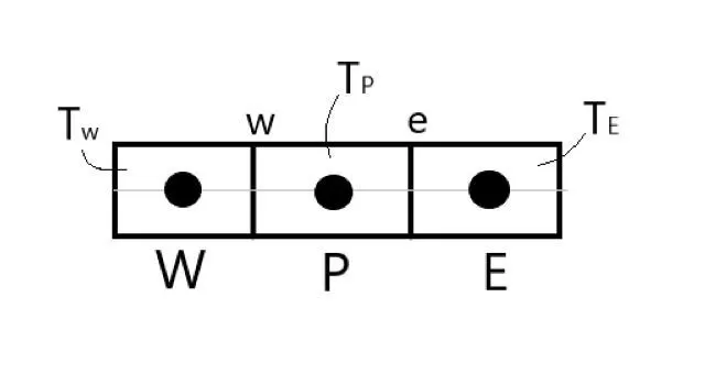
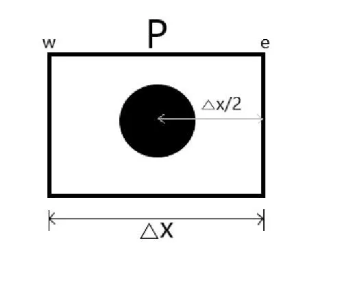
The entire volume is discretized into smaller control volumes as shown in the above image. Let us consider that each volume is formed by the combination of several small volumes dv. Now on that small volume dv,
`del/(delx) *(alpha(delT)/(delx)) + S = 0`
Thus for total volume, the value at the small volume dv is multiplicated and integrated as follow,
`int(del/(delx) *(alpha(delT)/(delx)) + S)dv = 0`
`int_w^edel/(delx)*(alpha(delT)/(delx))dv + intS dv =0`
Let us consider, dv = A.dx,
`=> int_w^edel/(delx)*(alpha(delT)/(delx))A dx + intS dv =0`
we know that `intd/(dx)(f)dx = f`
`=> [alpha A(delT)/(delx)]_w^e + barSdv=0` `[because`avg S (`barS`) * total volume = `intSdv`]
where `barS` is the average value of the source term.
By applying higher and lower limits,
`=> alpha_eA ((delT)/(delx))_e - alpha_wA((delT)/(delx))_w+barS dv = 0`
The `(delT)/(delx)` term can be found by implementing the taylor series of 1st order or 2nd order approximations.
`=> alpha_eA[(T_E - T_P)/(Deltax)]- alpha_wA[(T_P-T_W)/(Deltax)]+barSdv = 0` `->2`
The limits are applied to `alpha`, since the thermal diffusivity changes with respect to temperature and it should be linearize. The `barSdv`term should also be linearized. The source term is in the nonlinear form. The nolinear terms should be linearized to get the converged results. The stability and convergence of linearized terms are at high level when compared with non linear term.
The equation 2 can be written as,
[Heat flux out] - [heat flux in] + Source term = 0.
Thus, the above equation explains that the amount of heat in the volume is conserved.
Different schemes in FVM:
Gradient scheme:
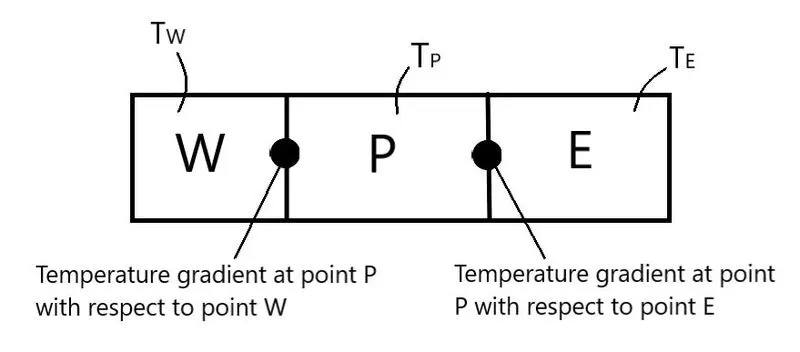
The gradient scheme is a scheme used to solve the equations in the finite volume method. In gradient scheme, the required term in a particular volume is solved with respect to the values of the neighbouring volumes. In the above example, the temperature gradient at the volume P is solved with the help of gradient scheme by considering the temperature of the neighbouring volumes.
Interpolation scheme:
Interpolation scheme is an important scheme to solve the equation in the FVM. The interpolation scheme is used to In the above example, the temperature gradient term can be found or solved with the help of temperatures in the neighbouring volumes. The temperature term at the gradient point can be obtained by applying various interpolation schemes. This scheme is also employed to get the face values of `phi` and `(delphi)/(delx)` by making some assumptions.
Types of interpolation scheme:
1. Upwind interpolation scheme
2. Linear interpolation scheme
3. Quadratic upwind interpolation scheme (QUICK)
4. Hybrid difference scheme
5. Total variation diminishing scheme (TVD)
Upwind interpolation scheme - This interpolation scheme is similar to that of backward or forward finite difference approximation. This scheme approximate the value of some variables at the east face of the control volume.
Linear interpolation scheme - This scheme is similar to the central difference scheme. In this scheme, the variables at centre are found by applying the linear interpolation method of values at the two nearest nodes.
Quadratic upwind interpolation scheme (QUICK) - This scheme derived the variables by using polynomial fitting. This scheme is third order accurate and it prones to oscillations.
Hybrid difference scheme - The hybrid difference scheme is the combination of both central difference scheme and upwind difference scheme. This scheme is used to find the numerical solution of convection-diffusion problems.
Total variation diminishing scheme (TVD) - This scheme is used for solving the hyperbolic partial differential equation in certain discretization schemes. It has a good role in the CFD domain.
Flux limiter:
The flux limiters are used in the high resolution schemes. The high resolution schemes are the solving method to solve the partial differential equation where the high accuracy was needed even there may be a shock or discontinuities. The specious oscillations due to shock or discontinuities and the sharp changes in domain can be minimised by using the flux limiters in solving the high resolution schemes. The total variation diminishing solution may occur when the flux limiters are applied with high resolution scheme to solve the problems.
The spatial derivatives can be converted into the realistic values by using the flux limiters. This is the major concept behind the construction of flux limiter schemes. The flux limiters are used in the problems having sharp wave fronts. Let us consider a 1D semi discrete scheme,
`(du_i)/dt + 1/(Deltax_i)[F (u_(i+(1)/2))-F(u_(i-(1)/2))] = 0`
where, `F (u_(i+(1)/2)) and F (u_(i-(1)/2))` are the edge fluxes. Based on the higher or lower resolution schemes, the flux limiter changes these edge fluxes as follow,
`F (u_(i+(1)/2)) = f_(i+(1)/2)^(low) - phi(r_i)(f_(i+(1)/2)^(low)-f_(i+(1)/2)^(high))` and
`F (u_(i-(1)/2)) = f_(i-(1)/2)^(low) - phi(r_(i -1) )(f_(i-(1)/2)^(low)-f_(i-(1)/2)^(high))`. Depending upon the colseness of the gradient in the particular cell, this switch was made by the flux limiter.
In the above equations, `f^(low)`= low resolution flux
`f^(high)` = high resolution flux
`phi(r)` = flux limiter function
r = ratio of successive gradients on the solution mesh
`r_i = (u_i - u_(i-1))/(u_(i+1)-u_i)`
The flux limiter function should either be equal to zero or greater than zero (`phi(r) >= 0`). If `phi(r) = 0`, then the flux is represented by low resolution scheme. If `phi(r) =1`, then the flux is represented as high resolution scheme.
Conclusion:
Thus, the finite volume method is the most efficient and accurate method in solving the problems in computational fluid dynamics (CFD).
Keywords:
Finite volume method, finite difference method, boundary element method, finite element method, flux limiter, Upwind interpolation scheme, Linear interpolation scheme, Quadratic upwind interpolation scheme (QUICK), Hybrid difference scheme, Total variation diminishing scheme (TVD).
Reference: