FSAE Car Project
Introduction
The objective of the current study is to simulate air flow over a standard FSAE vehicle. Two different cases with different track conditions are analyzed in depth. The drag and downforce components acting on the different components of the vehicle are measured and plotted for both cases.
An FSAE vehicle is designed to enhance the efficiency of the vehicle by making optimal use of the aerodynamic forces acting on it. Two of the primary aerodynamic forces acting on an FSAE vehicle are the Drag and Lift forces. Unlike an airfoil, automobiles are designed to generated a negative lift, also known as the downforce, to ensure the vehicle stays in contact with the ground. These two forces are calculated as shown below:
`D=1/2*rho*A*v^2*Cd`_______________i
`L=1/2*rho*A*v^2*Cl`_______________ii
where `D` is the Drag Force, `L` is the Lift force, `rho` is the density of the fluid, `A` is the acting area of the fluid, `v` is the free stream velocity of the fluid, `Cd` and `Cl` refer to the drag and lift coefficients respectively.
The design of an FSAE vehicle is optimized to increase downforce and reduce drag. The downforce is primarily responsible for the grip generated by an FSAE vehicle, allowing it to move around corners at fast speeds while experiencing high centrifugal forces. The front wing of the FSAE vehicle is modelled along the lines of an inverted airfoil to generate downforce instead of lift. The relatively lower height of the underbody makes use of the choked venturi effect, allowing the development of a low pressure and high velocity region below
Computational Details and Case Setup
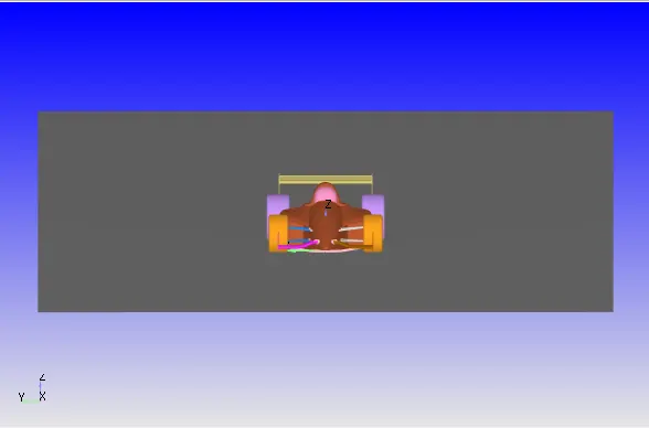
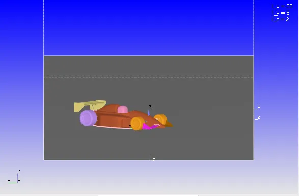
The FSAE geometry, that was provided in the challenge, was imported into Converge Studio, which is used as a pre-processor and meshing software in the current study. The geometry is cleaned up to eliminate the intersecting and overlapping triangle errors. The FSAE geometry is placed inside a rectangular wind tunnel with dimensions of 25 x 5 x 2 m. The boundaries are flagged as shown in the table below
| Boundary Name | Condition |
| body | Wall: Law of Wall, TKE: Ne, Omega: Wall Model |
| rear_wing | Wall: Law of Wall, TKE: Ne, Omega: Wall Model |
| front_wheels | Wall: Law of Wall, TKE: Ne, Omega: Wall Model |
| rear_wheels | Wall: Law of Wall, TKE: Ne, Omega: Wall Model |
| front_suspension_right | Wall: Law of Wall, TKE: Ne, Omega: Wall Model |
| front_suspension_left | Wall: Law of Wall, TKE: Ne, Omega: Wall Model |
| rear_suspension_right | Wall: Law of Wall, TKE: Ne, Omega: Wall Model |
| rear_suspension_left | Wall: Law of Wall, TKE: Ne, Omega: Wall Model |
| front_wing_right | Wall: Law of Wall, TKE: Ne, Omega: Wall Model |
| front_wing_left | Wall: Law of Wall, TKE: Ne, Omega: Wall Model |
| underbody | Wall: Law of Wall, TKE: Ne, Omega: Wall Model |
| inlet | Inflow: Axial velocity: DI, Pressure: NE |
| outlet | Outflow: Axial velocity NE, Pressure=101325 Pa |
| symmetry | Symmetry |
| bottom | Wall: Law of Wall, TKE: Ne, Omega: Wall Model |
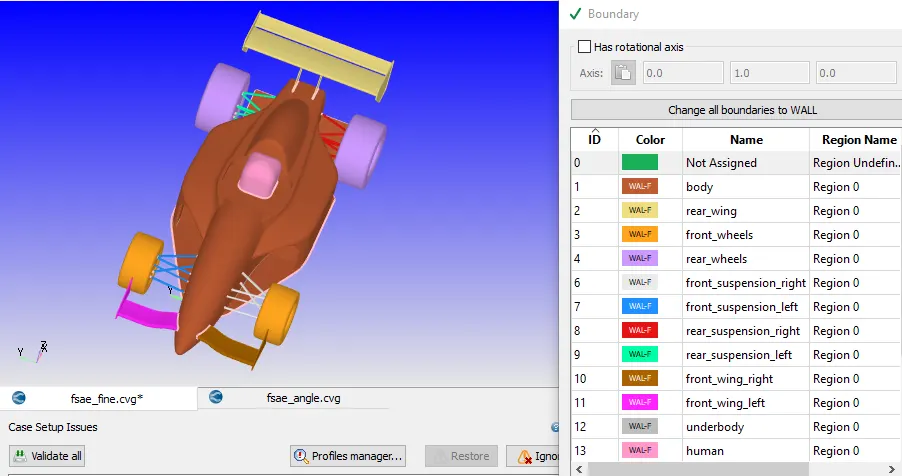
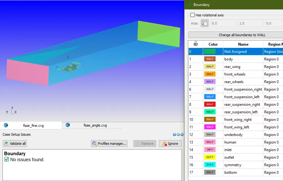
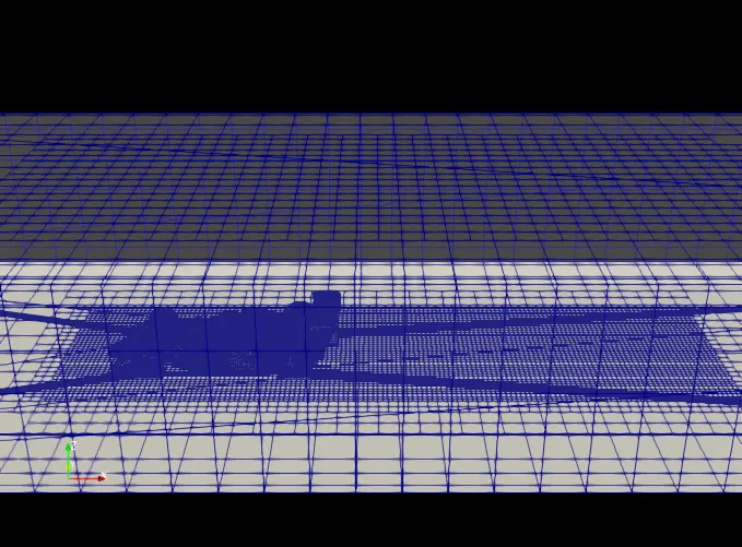
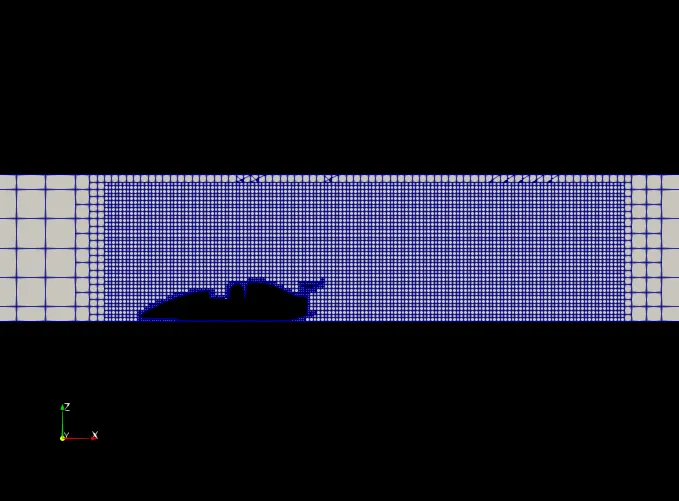
The standard `k-omega` turbulence model has been adopted for the current study. Since the drag and lift forces are primarily studied in the viscous sublayer and buffer region, it is logical to opt for a turbulence model that accurately predicts wall behaviours for low values of Y+. A Y+ of <30 is desired, and as per the pointwise mesh generator, a base mesh size 0.028 m is desirable with an embedding scale of 5. However, due to computational restrictions, a structured mesh with a base gid size of 0.4 m is chosen. To improve the accuracy of the obtained results, boundary embedding is applied on the FSAE vehicle at a scale of 4 and a box embedding is applied around the vehicle at a scale of 3 to study the wake formation, as shown below. Total cell count was roughly ~400,000 cells.
As per the challenge, analysis of two separate cases is required.
Case 1: Straight track with an average speed of 75 km/hr (20.83 m/s)
Case 2: Lots of turns (70 % x 45º, 20 % x 80º, 10 % x 20º) at an average speed of 45 km/hr (12.5 m/s). An average angle of 49.5º is obtained. As a result, the FSAE vehicle is oriented accordingly with the direction of the axial flow, as shown below.
A fully hydrodynamic, compressible, transient solver operating on the PISO algorithm is chosen for both cases. The total flow time for both cases is calculated as 3*Mean flow time, which is shown below
Case 1: 3*25/20.83=3.6 s
Case 2: 3* 25/12.5= 6 s
Results and Discussion
Case 1
Preliminary observations from the velocity and pressure contours of the FSAE vehicle suggest the development of a strong axial drag force along the tyres and human. This can be attributed to the fact that the free stream air comes in direct axial contact and loses most of its kinetic energy, which is exerted as a drag force. However, the geometry of the vehicle body directs the flow upwards, leading to a jump in the free stream velocity and development of a low pressure zone in the axial direction. This significantly reduces the drag force exerted.
Case 2
Unlike the contours shown above, the axis of the vehicle is not parallel to the free stream velocity of the air. As a result, there might be slight reduction in the axial drag due to a reduction of the cross-section area exposed to the axial streamlines of the air. However, this might lead to the development of a weak sideforce due to the centrifugal effect, as clearly evident by the difference in the pressure along the windward and leeward sides of the vehicle.
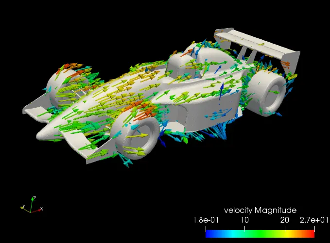
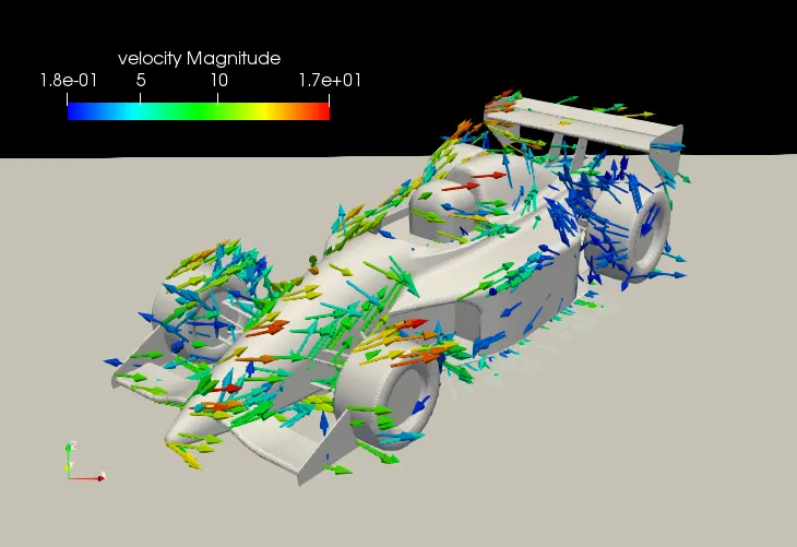
Both cases, however, presented interesting aspects of the geometry of the FSAE vehicle. For instance, the windward portion of the vehicle (in front of the human) is designed in such a way so as to promote flow separation while the car is travelling along a straight track or while taking a turn. This flow separation diverts the flow of the air above the vehicle, reducing drag significantly. It is interesting to note that this flow separation near the rear wing leads to recirculation, which might exert a positive lift force on the rear wing. To further confirm the presence of recirculation, velocity streamlines for both cases were plotted as shown below. Both cases chaotic recirculation in the wake region, which suggests that there might be a positive lift component being exerted on the rear wing. It is also noteworthy that there seems to be minimal vortex formation below the body of the vehicle. Since vortices flow in the direction of the fluid flow, the end plates of the front ensure that these vortices are diverted from the underbody of the vehicle. This improves the stability of the vehicle and gives it a significant performance enhancement.
Analysis of Drag and Downforce
The following graphs show the transient variation of the Drag and Downforce for both cases. Assuming the body and the underbody of the vehicle to be separate entities, the magnitude of drag acting on the body and underbody are maximum for both cases. However, as a result of the venturi effect, a negative drag acts on the underbody in both cases--which neutralises the positive drag exerted on the main body. It can be observed that the magnitude of drag for Case 1 is ~5500 N and for Case 2 is ~3600 N. This difference is attributed to the inclination of the car with respect to the free stream velocity of the air and the lower free stream velocity of the air. The cross sectional area of the body and underbody exposed to the free stream of air in case of the inclined orientation is lesser than in Case 1, leading to a lower drag force for Case 2. Furthermore, the lower free stream velocity in Case 2 also leads to a weaker drag force than in Case 1. It is notable that the Downforce remains the same, since there is no alteration in the wing angles. Similar observations are made in case of the front and rear wheels, which report relatively lower drag values in Case 2 than in Case 1.
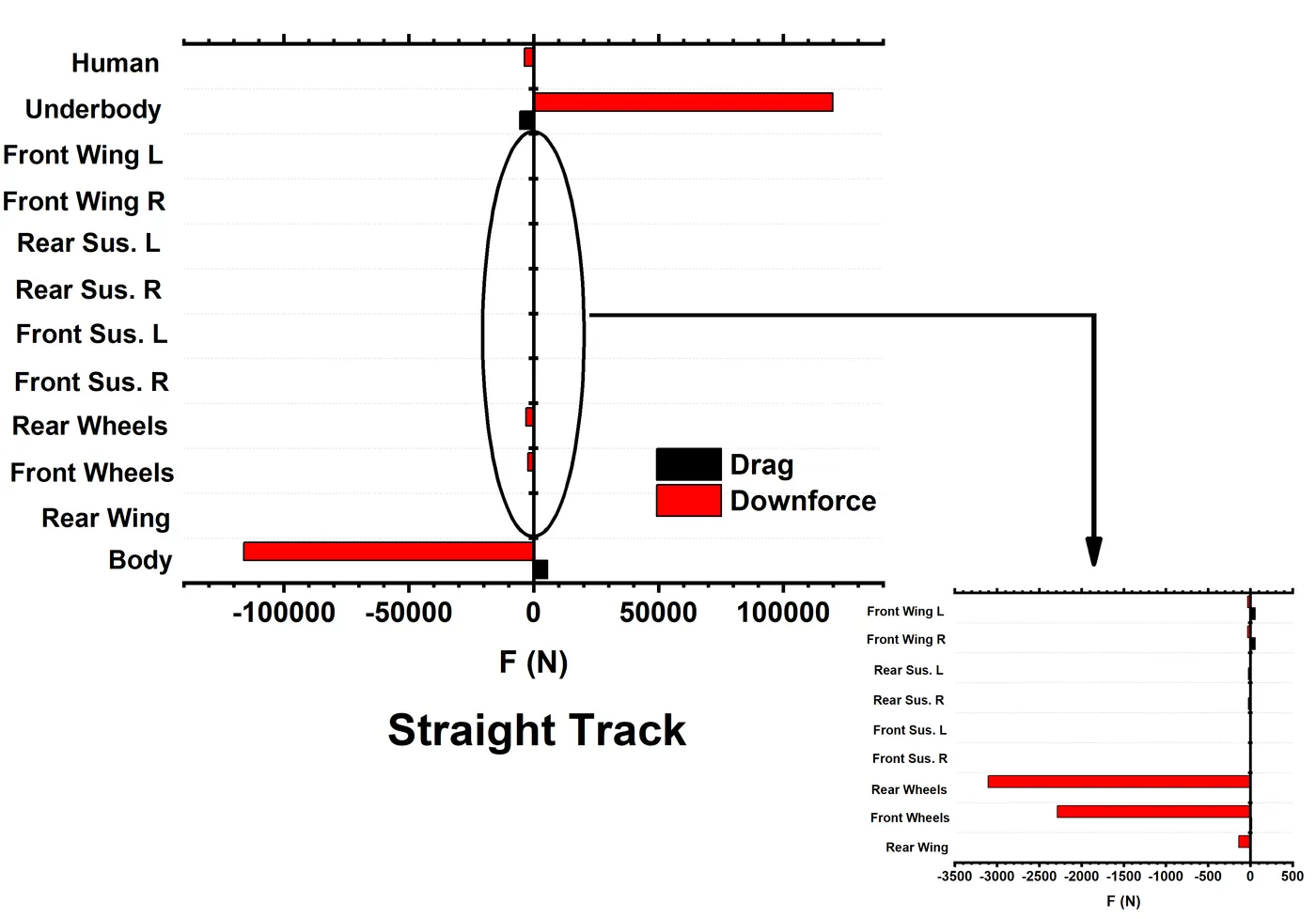
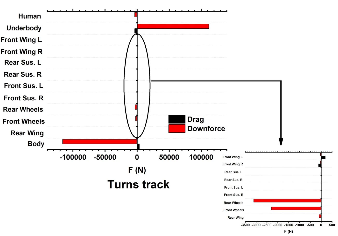
There is a slight variation in the drag values reported for the suspension links in both cases. The front and rear suspension links reported drag forces of 4.4 N and -20.8 N respectively for both, the left and right sides. The negative drag force on the rear suspension links can be attributed to the effect of air recirculation behind the rear wing in the wake, which creates a partial vacuum and results in the exertion of a minute negative pressure on the suspension links. However, Case 2 reports different drag values for the left and right suspension links in the front and rear ends of the vehicle due to its asymmetric orientation.
The average values of Y+ obtained for Case 1 was 350 while Case 2 reported values of 450. These are significantly higher than the desired values of Y+<30, which is attributed to the coarse mesh due to the computational restrictions. These values suggest that while the simulation might give an approximate idea about the behaviour of the vehicle, there might be significant changes in the drag and downforce values upon mesh refinement.
Conclusion
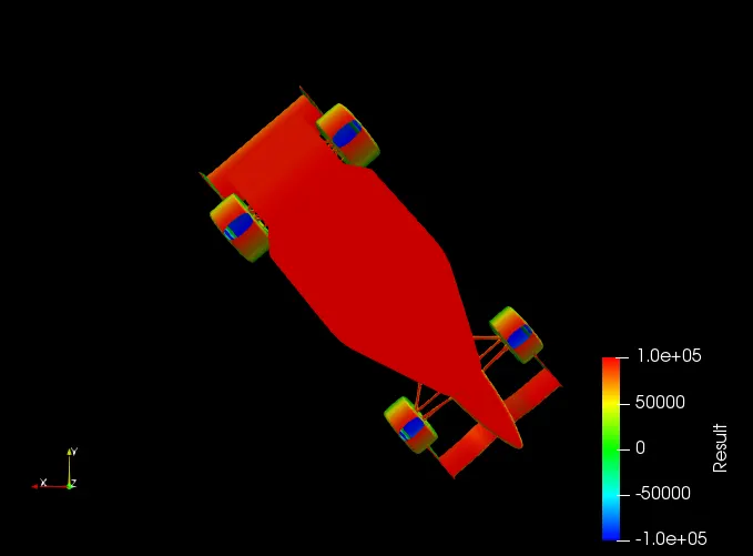
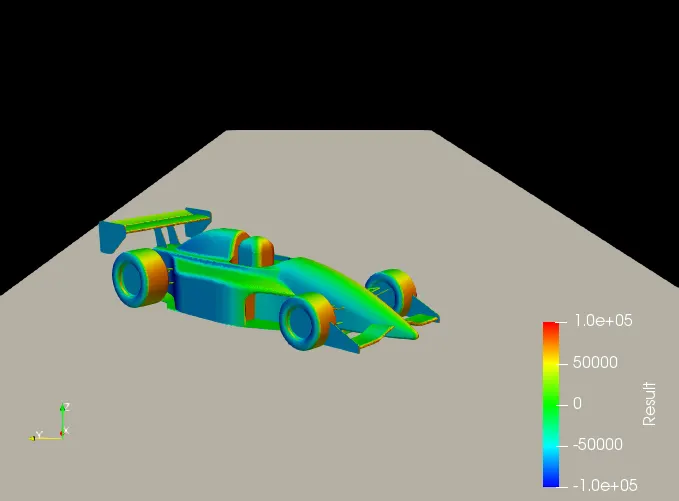
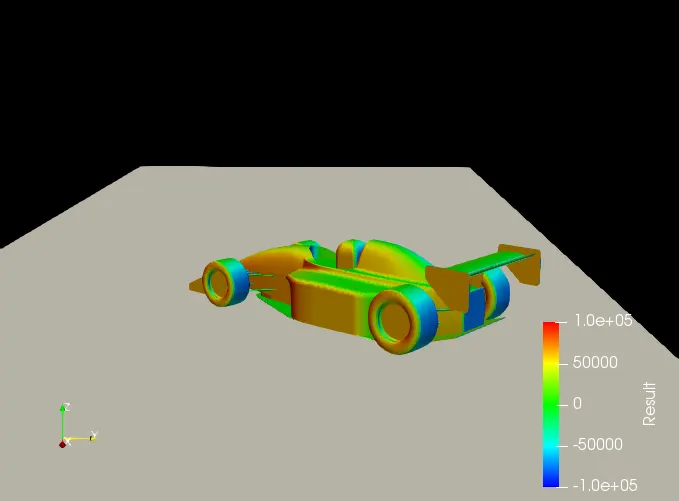
The table given below summarises the net values of the forces acting on the FSAE vehicle, with the contours shown below. While the desired effect is achieved with a lower drag force and a high downforce, these values need significant improvement for competitive racing, especially for Case 2. For the vehicle to carry out cornering at high speeds, it is essential to generate a higher downforce than it does while driving on straights to improve grip and traction. Similarly, a significant drag reduction is expected in Case 2, given that there is a reduction of almost ~8.3 m/s in the free stream velocity It is noteworthy that due to the orientation of the vehicle in Case 2, it was crucial to study the effect of the sideforces acting on the body due to the centrifugal effect, which, as expect, was found to be 0 in Case 1.
| Force | Case 1: Straight track | Case 2: Turns |
| Drag (N) | 69 | 60 |
| Downforce (N) | -5411 N | -5400 |
| Side force (N) | 0 | 30 N |
Case 1: Straight track
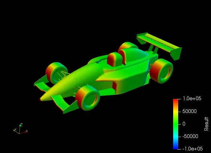
Drag Force
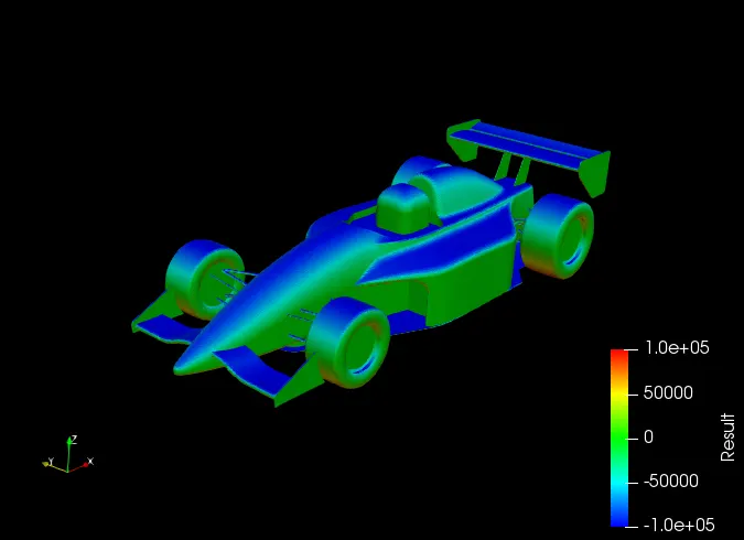
Downforce_part a.
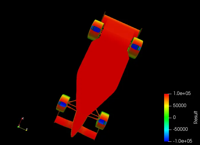
Downforce_part b.
Case 2: Track with turns
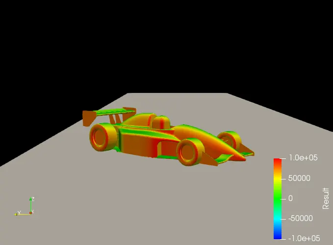
Drag_part a.
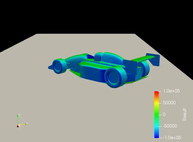
Drag_part b.
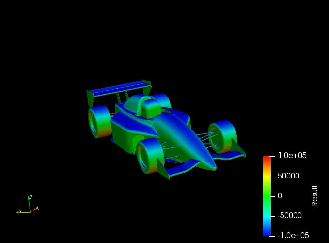
Downforce_part a.
Downforce_ part b.
Sideforce_part a.
Sideforce_part b.