Frequency determination and Bump oscillation profile for Curb, Design & GVW conditions

GIVEN DATA:

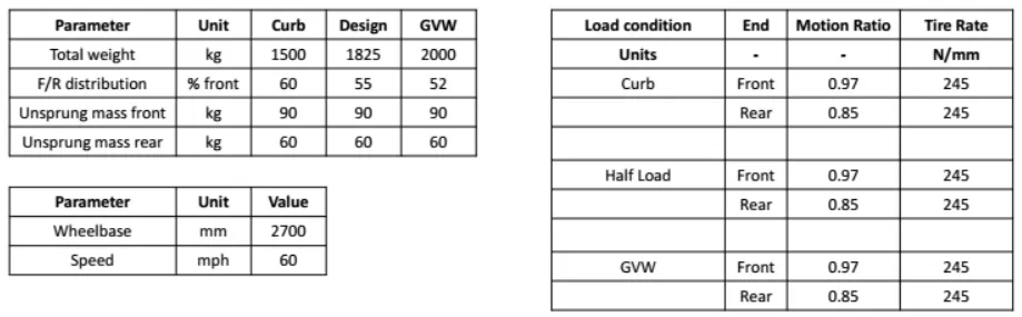
SOLUTION:

Workflow:

- Fix the spring rates

- Find the ride rate using front sprung mass frequency (given)

- Find the rear sprung mass frequency using time-lag (given)

- Find unsprung mass frequency using tire rate and wheel rate

- Find the frequency ratio for all conditions

Abbreviations:

`k_w` = wheel rate (N/mm) `k_t` = tire rate (N/mm) `k_s` = spring rate (N/mm) `k_r` = ride rate (N/mm) `MR` = motion ratio

Suffix: `f` = front `r` = rear

(i) Recommended rear sprung mass frequency based on speed and wheelbase at half load condition

`f_f = 1.15 Hz`

`t_f = frac[1][f_f] = frac[1][1.15] = 0.869 sec`

`t_[de lay] = frac[wheelbase][speed] = frac[frac[2700][1000]][60.(0.44704)] = 0.1 sec` ... `:' 1 mph = 0.44704 m/sec`

`t_[de lay] = t_f - t_r rArr 0.1 = 0.869 - t_r rArr t_r = 0.769 sec`

`f_r = frac[1][t_r] = frac[1][0.769] = 1.3004 sec`

(ii) Front sprung mass natural frequency at half load = 1.15 Hz

(iii) Front spring rate

Sprung Mass Frequency (Front),

`f_[s f] = 1/[2pi] sqrt[k_[r f]/m_sf]`

`1.15 = 1/[2pi] sqrt frac[k_[r f] *10^3][456.875]`

`k_[r f] = 23.85353845 N/[mm]`

Ride rate (Front),

`k_[r f] = frac[k_[w f] . k_t][k_[w f] + k_t]`

`23.85353845 = frac[k_[w f] . 245][k_[w f] + 245]`

`k_[w f] = 26.42645457 N/[mm]`

`k_[w f] = k_[s f] . (MR_f)^2`

`26.42645457 = k_[s f]. 0.97^2`

`k_[s f] = 28.08635835 N/[mm]` ... Front spring rate

(iv) Rear spring rate

Sprung Mass Frequency (Rear),

`f_[s r] = 1/[2pi] sqrt[k_[rr]/m_[sr]]`

`1.3004 = 1/[2pi] sqrt frac[k_[rr] *10^3][380.625]`

`k_[rr] = 25.4103688 N/[mm]`

Ride rate (Rear),

`k_[rr] = frac[k_[w r] . k_t][k_[w r] + k_t]`

`25.4103688 = frac[k_[w r] . 245][k_[w r] + 245]`

`k_[w r] = 28.35079381 N/[mm]`

`k_[w r] = k_[s r] . (MR_r)^2`

`28.35079381 = k_[s r]. 0.85^2`

`k_[s r] = 39.23985302 N/[mm]` ... Rear spring rate

(v) Front sprung mass natural frequencies at curb and GVW = 1.221272893 Hz, 1.127699595 Hz

(vi) Rear sprung mass natural frequencies at curb and GVW = 1.543787164 Hz, 1.195812396 Hz

(vii) Front unsprung mass natural frequency at all three load conditions = 12.3967422 Hz

(viii) Rear unsprung mass natural frequency at all three load conditions = 15.4897954 Hz

(ix) Rear/Front frequency ratio for all three load conditions

Frequency ratio	Curb	Design	GVW
Sprung mass	1.26408043	1.130782609	1.060399773
Unsprung mass	1.249505325	1.249505325	1.249505325

Excel Output:

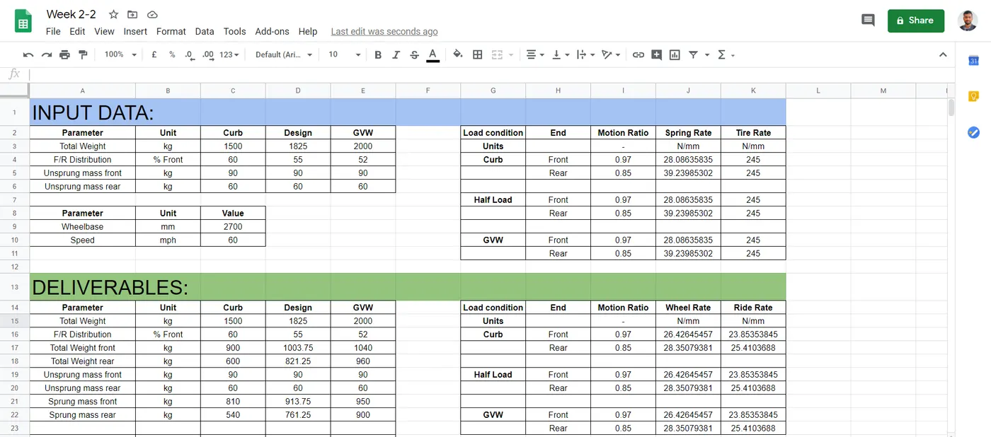
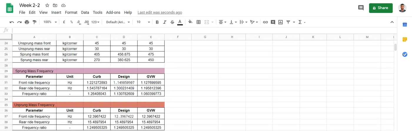
Excel Link: https://docs.google.com/spreadsheets/d/1zqyGgVErN-9mrssG2wOUOlMIueMbVkzQtySxO5IsP0c/edit#gid=0

AIM:

2. Plot the bump oscillation profile for all three load conditions using the method we developed in class. Submit the code.

SOLUTION:

Formulae:

Amplitude Front = `e^(-t) . sin(2 pi f t)`

Amplitude Rear = `e^(-t) . sin(2 pi f (t - t_d))`

`t_d` = Delay time (secs)

Curb condition:

Code #1:

% Curb condition.

% Inputs:

Ws_front = 405; Ws_rear = 270;  % Sprung mass (kg/corner)
Wus_front = 45; Wus_rear = 30;  % Unsprung mass (kg/corner)

kt_front = 245; kt_rear = 245;  % Tire rate (N/mm)
kw_front = 26.42645457; kw_rear = 28.35079381;  % Wheel rate(N/mm)
kr_front = 23.85353845; kr_rear = 25.4103688;   % Ride rate (N/mm)

t_d = 0.1006;   % Time Delay (sec)


% Solution:

fs_front = sqrt(kr_front*1000/Ws_front)/(2*pi); % Sprung mass frequency (Hz)
fs_rear = sqrt(kr_rear*1000/Ws_rear)/(2*pi);

fus_front = sqrt((kt_front + kw_front)*1000/Wus_front)/(2*pi);  % Unsprung mass frequency (Hz)
fus_rear = sqrt((kt_rear + kw_rear)*1000/Wus_rear)/(2*pi);

time = linspace(0,3.5,350);  % Time period

for i = 1:length(time)
    amp_s_front(i) = exp(-time(i))*sin(2*pi*fs_front.*time(i));
    amp_s_rear(i) = exp(-time(i))*sin(2*pi*fs_rear.*(time(i)-t_d));
    amp_us_front(i) = exp(-time(i))*sin(2*pi*fus_front.*time(i));
    amp_us_rear(i) = exp(-time(i))*sin(2*pi*fus_rear.*(time(i)-t_d));
end


% Plot:

figure(1)
subplot(2,1,1)
plot(time,amp_s_front,'linewidth',3);
hold on
plot(time,amp_s_rear,'linewidth',3);
title('Bump Oscillation at Curb condition (Sprung)')
xlabel('Time (sec)')
ylabel('Amplitude (m)')
grid on

subplot(2,1,2)
plot(time,amp_us_front,'linewidth',3);
hold on
plot(time,amp_us_rear,'linewidth',3);
title('Bump Oscillation at Curb condition (Unsprung)')
xlabel('Time (sec)')
ylabel('Amplitude (m)')
grid on

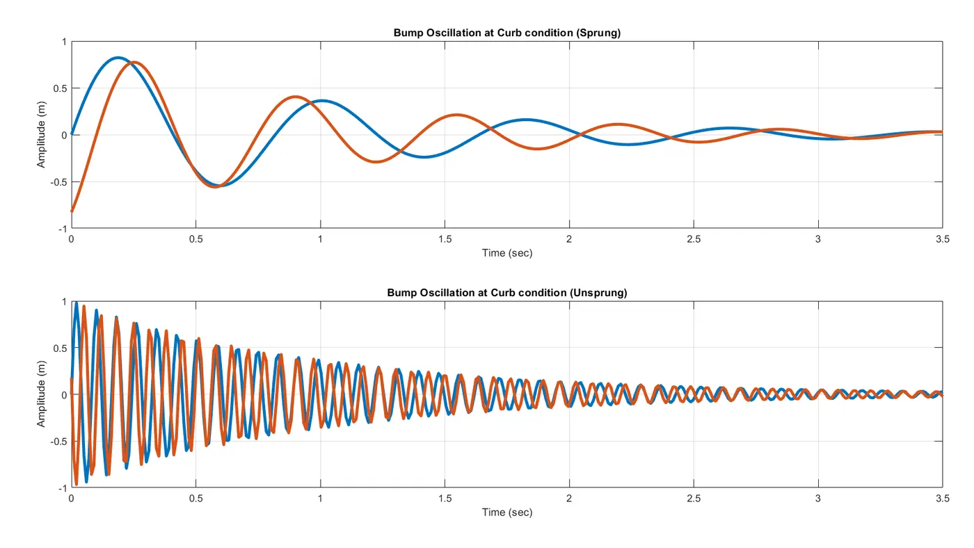
Output #1:

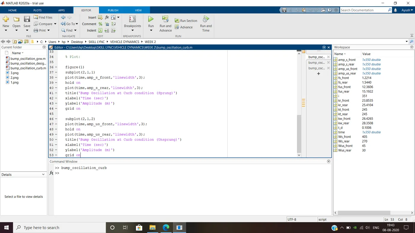
Plot #1:

Design condition:

Code #2:

% Design condition.

% Inputs:

Ws_front = 456.875; Ws_rear = 380.625;  % Sprung mass (kg/corner)
Wus_front = 45; Wus_rear = 30;  % Unsprung mass (kg/corner)

kt_front = 245; kt_rear = 245;  % Tire rate (N/mm)
kw_front = 26.42645457; kw_rear = 28.35079381;  % Wheel rate(N/mm)
kr_front = 23.85353845; kr_rear = 25.4103688;   % Ride rate (N/mm)

t_d = 0.1006;   % Time Delay (sec)


% Solution:

fs_front = sqrt(kr_front*1000/Ws_front)/(2*pi); % Sprung mass frequency (Hz)
fs_rear = sqrt(kr_rear*1000/Ws_rear)/(2*pi);

fus_front = sqrt((kt_front + kw_front)*1000/Wus_front)/(2*pi);  % Unsprung mass frequency (Hz)
fus_rear = sqrt((kt_rear + kw_rear)*1000/Wus_rear)/(2*pi);

time = linspace(0,3.5,350);  % Time period

for i = 1:length(time)
    amp_s_front(i) = exp(-time(i))*sin(2*pi*fs_front.*time(i));
    amp_s_rear(i) = exp(-time(i))*sin(2*pi*fs_rear.*(time(i)-t_d));
    amp_us_front(i) = exp(-time(i))*sin(2*pi*fus_front.*time(i));
    amp_us_rear(i) = exp(-time(i))*sin(2*pi*fus_rear.*(time(i)-t_d));
end


% Plot:

figure(2)
subplot(2,1,1)
plot(time,amp_s_front,'linewidth',3,'color','g');
hold on
plot(time,amp_s_rear,'linewidth',3,'color','y');
title('Bump Oscillation at Design condition (Sprung)')
xlabel('Time (sec)')
ylabel('Amplitude (m)')
grid on

subplot(2,1,2)
plot(time,amp_us_front,'linewidth',3,'color','g');
hold on
plot(time,amp_us_rear,'linewidth',3,'color','y');
title('Bump Oscillation at Design condition (Unsprung)')
xlabel('Time (sec)')
ylabel('Amplitude (m)')
grid on

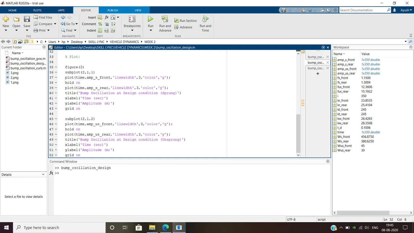
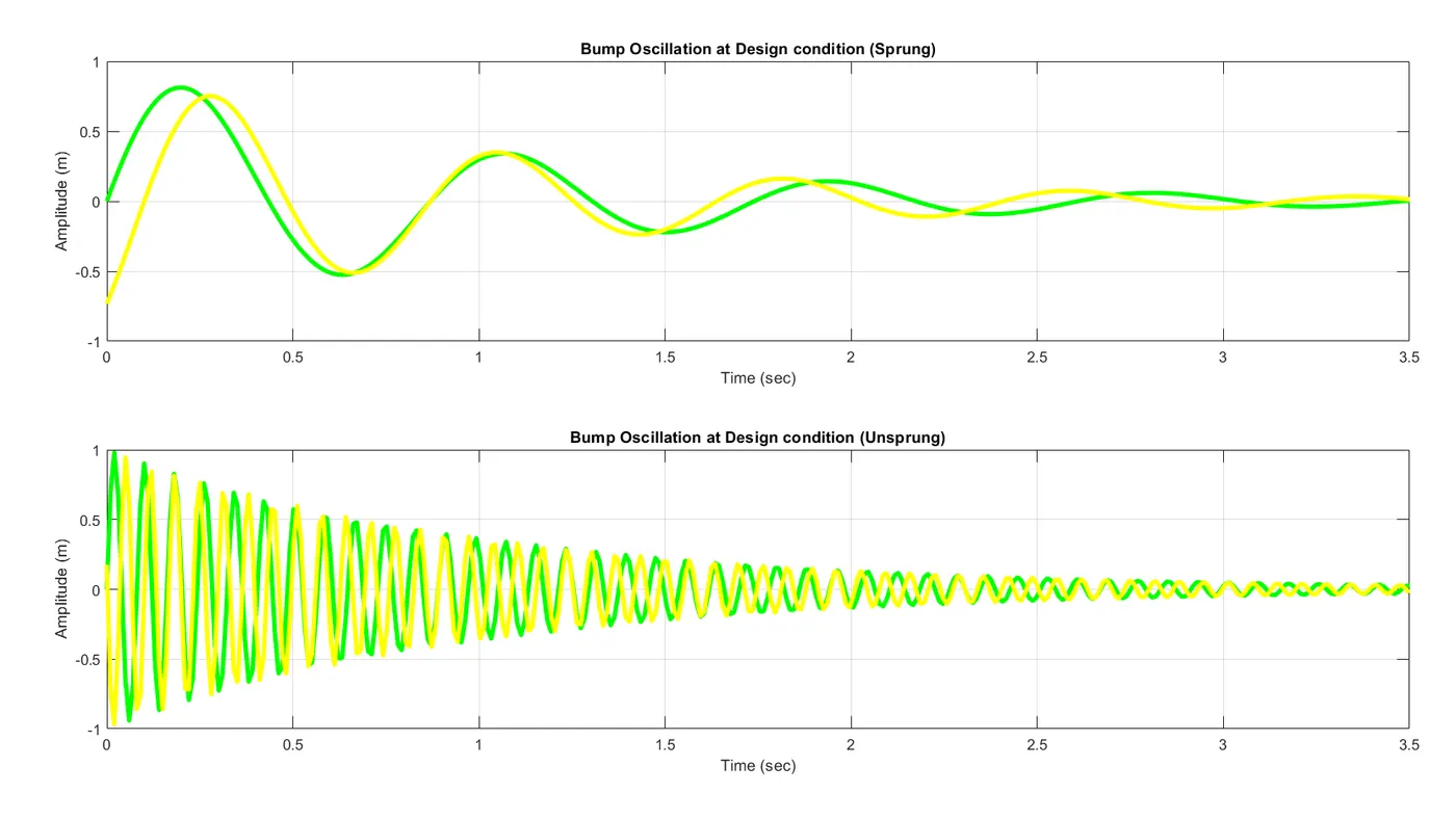
Output #2:

Plot #2:

GVW condition:

Code #3:

% GVW condition.


% Inputs:

Ws_front = 475; Ws_rear = 450;  % Sprung mass (kg/corner)
Wus_front = 45; Wus_rear = 30;  % Unsprung mass (kg/corner)

kt_front = 245; kt_rear = 245;  % Tire rate (N/mm)
kw_front = 26.42645457; kw_rear = 28.35079381;  % Wheel rate(N/mm)
kr_front = 23.85353845; kr_rear = 25.4103688;   % Ride rate (N/mm)

t_d = 0.1006;   % Time Delay (sec)


% Solution:

fs_front = sqrt(kr_front*1000/Ws_front)/(2*pi); % Sprung mass frequency (Hz)
fs_rear = sqrt(kr_rear*1000/Ws_rear)/(2*pi);

fus_front = sqrt((kt_front + kw_front)*1000/Wus_front)/(2*pi);  % Unsprung mass frequency (Hz)
fus_rear = sqrt((kt_rear + kw_rear)*1000/Wus_rear)/(2*pi);

time = linspace(0,3.5,350);  % Time period

for i = 1:length(time)
    amp_s_front(i) = exp(-time(i))*sin(2*pi*fs_front.*time(i));
    amp_s_rear(i) = exp(-time(i))*sin(2*pi*fs_rear.*(time(i)-t_d));
    amp_us_front(i) = exp(-time(i))*sin(2*pi*fus_front.*time(i));
    amp_us_rear(i) = exp(-time(i))*sin(2*pi*fus_rear.*(time(i)-t_d));
end


% Plot:

figure(3)
subplot(2,1,1)
plot(time,amp_s_front,'linewidth',3,'color','k');
hold on
plot(time,amp_s_rear,'linewidth',3,'color','c');
title('Bump Oscillation at GVW condition (Sprung)')
xlabel('Time (sec)')
ylabel('Amplitude (m)')
grid on

subplot(2,1,2)
plot(time,amp_us_front,'linewidth',3,'color','k');
hold on
plot(time,amp_us_rear,'linewidth',3,'color','c');
title('Bump Oscillation at GVW condition (Unsprung)')
xlabel('Time (sec)')
ylabel('Amplitude (m)')
grid on

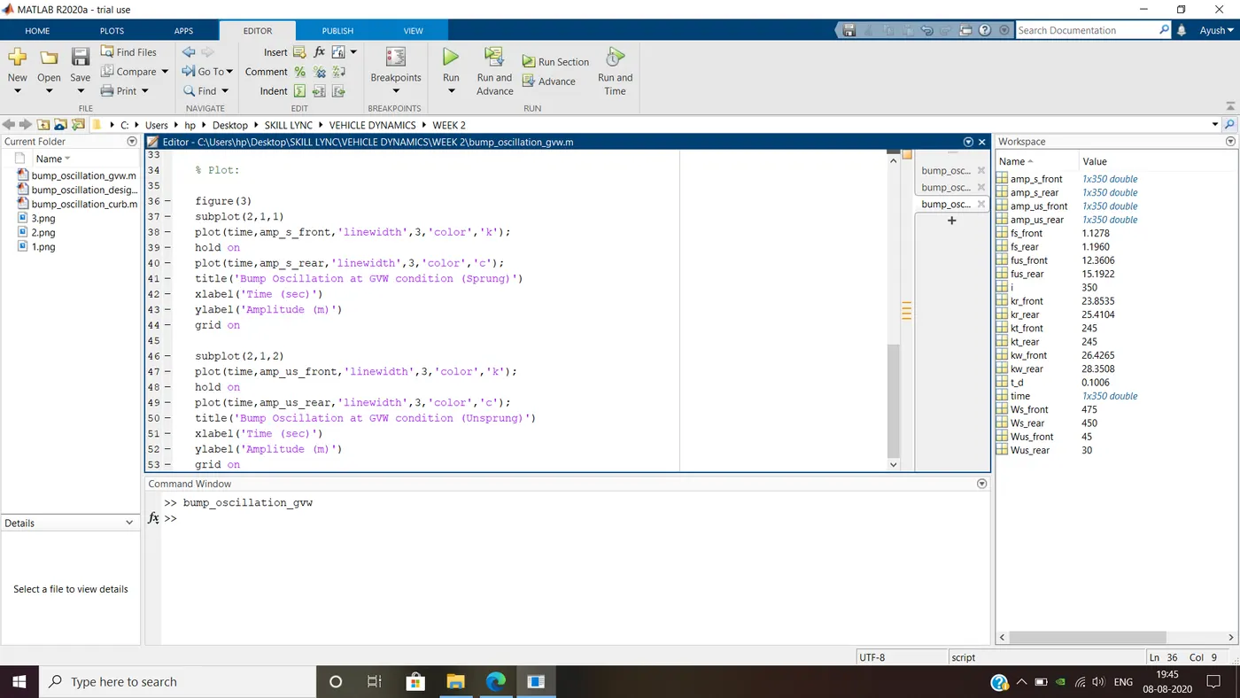
Output #3:

Plot #3:

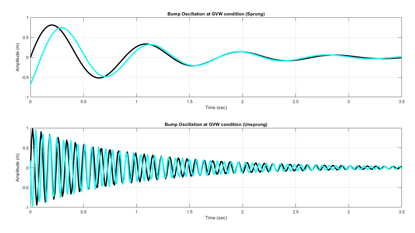
CONCLUSION: From the above results, we can infer that the bump oscillation profile is considerably optimized (in-phase) for the initial cycle in both Design and GVW conditions. We don't worry much about the Curb condition as the vehicle is empty in that case (not a practical scenario.