Final Project: Design of an Electric Vehicle
Aim: - Design of an electric vehicle using MATLAB model of an electric car using lithium-ion battery and an induction motor. Choose suitable blocks from the powertrain blockset.
Introduction: -
n electric vehicle (EV) is a vehicle that uses one or more electric motors or traction motors for propulsion. An electric vehicle may be powered through a collector system by electricity from off-vehicle sources, or may be self-contained with a battery, solar panels, fuel cells or an electric generator to convert fuel to electricity. EVs include, but are not limited to, road and rail vehicles, surface and underwater vessels, electric aircraft and electric spacecraft.
EVs first came into existence in the mid-19th century, when electricity was among the preferred methods for motor vehicle propulsion, providing a level of comfort and ease of operation that could not be achieved by the gasoline cars of the time. Modern internal combustion engines have been the dominant propulsion method for motor vehicles for almost 100 years, but electric power has remained commonplace in other vehicle types, such as trains and smaller vehicles of all types.
Commonly, the term EV is used to refer to an electric car. In the 21st century, EVs have seen a resurgence due to technological developments, and an increased focus on renewable energy and the potential reduction of transportation's impact on climate change and other environmental issues. Project Drawdown describes electric vehicles as one of the 100 best contemporary solutions for addressing climate change.
Types of EVs
EVs (also known as plug-in electric vehicles) derive all or part of their power from electricity supplied by the electric grid. They include AEVs and PHEVs.
AEVs (all-electric vehicles) are powered by one or more electric motors. They receive electricity by plugging into the grid and store it in batteries. They consume no petroleum-based fuel and produce no tailpipe emissions. AEVs include Battery Electric Vehicles (BEVs) and Fuel Cell Electric Vehicles (FCEVs).
PHEVs (plug-in hybrid electric vehicles) use batteries to power an electric motor, plug into the electric grid to charge, and use a petroleum-based or alternative fuel to power the internal combustion engine. Some types of PHEVs are also called extended-range electric vehicles (EREVs).
System level configuration:
The major components forming the component system are
- Drive cycle
- Driver
- H-bridge
- DC motor
- Battery source
- Controlled PWM voltage
- Vehicle and others
The model of an EV in Simulink we need to model for mentioned component separately and then work together. All the main components are available in the library of Simulink blockset and we will be adding each component and configuring its parameter to fit the requirement of the model. Now the main vehicle body is to be modified.
Vehicle body
The vehicle body block consists of six ports used to model the various aspects of the vehicle body. The ports are mentioned below
H- this stands for ‘Hub’ and it connects hubs of the wheel to the main body.
V- stands for ‘Velocity; and is used to output speed/velocity of the vehicle when it is moving. It is a physical signal output port.
W-stands for ‘Headwind’ acting on the vehicle. It is physical signal input port.
NR- this is a physical output port to model the rear wheels normal forces
NF- this is a physical output port used to model the front wheel normal forces.
Beta- this is a physical signal input port and allows us to model the vehicle on an inclination angle to create the effect of a hill climbing force.
By double clicking the block we can modify the parameter as shown
We can modify various parameters of the vehicle body eg., Mass , No. of wheel per axle, distances of the centre of gravity to the front and rear axle. These are main parameters and have been left default values assigned when the block was added to the workspace. The next tab shows the parameter for drag
We can see from this image that the parameter of the frontal area, drag coefficient and air density can be modified in order to effect the drag force acting on the vehicle. In this case we have changed only drag coefficient to 0.5 from the default value 0.4 in order to model for the typical sedan. Air density and frontal area are normal from this type of vehicle.
Tires-
Tires used in EV are named as magic formula. There are several blocks but the magic formula block can be used to set longitudinal behaviors of vehicle tires on highway. Inertia, stiffness can also be modelled using this block.
The magic formula consists of the following 4 ports-
N- stands for ‘Normal’ . It is physical input port for normal force acting on tire and is considered in the positive direction.
S- stands for ‘Slip’. It is a physical output port and reports the slip acting on the vehicle.
- Stands for the ‘Axle’ and is a mechanical rotation conserving port for the wheel axle.
H- stands for hub and it is a mechanical translation conserving port for the wheel hub through which the thrust developed by the tires is applied to the vehicle body.
The image below shows the parameter for tire geometry. This is the only parameter modified and the value is set to 0.38
The next parameter is the dynamic of the magic formula. This is where we can model additional effects eg tire inertia and initial velocity.
Rolling resistance-
The rolling resistance parameters on the tires are chosen to switch ON the rolling resistance force on the tire. We have also selected rolling resistance to be 0.015 and velocity threshold to be 1e-3
The last parameter of the magic tire formula is the velocity threshold and this has been set to 0.1 m/s bellow this speed the block will not model any of the before mentioned effects of motion on to the tire hence it is called threshold velocity.
Gear-
Next the modelling of transmission system takes place. A simple gearbox block is used to simplify the transmission parameters. This block models the gear system with a fixed gear ratio and no inertia effect, however we can model the meshing of gear tooth. By double clicking we can set the parameters.
The main parameter for the dimple gear and follower is been set to 3.7 and also the output shaft rotates in the same direction as the input shaft.
Meshing loss-
The meshing loss selected follows a constant efficiency friction model with an efficiency of 0.82 and follower power threshold of 0.002W.
Side shaft-
An inertia block has been added to the workspace to provide an ideal mechanical rotational inertia for the simple gear block. This block has only one mechanical rotational conserving port and the positive direction of the block is from the port to the reference point which would be the simple gear in this case. The inertia torque acts in the positive direction and inertia accelerated to power directions.
The inertia block allows us to modify inertia and this parameter has been kept to a default value of 0.001.
Wind & slope
As mentioned, the velocity block allows us to model the effect of wind resistance and road inclination through the ‘w’ and beta ports respectively. In this model PS- constant block is used to model the parameter of wind and road inclination on the vehicles motion. For the wind effect we have given a constant signal of 5 m/s and this acts opposite to the direction of motion ie., head wind. For the road inclination we have given a constant signal of 0.
Velocity Subsystem-
The velocity port which outputs the velocity signal that is output from the velocity measured in miles per hour. To change these units, I have implemented a small subsystem from the output of the velocity port. The subsystem uses the following blocks-
PS- Simulink Converter- this block converts physical signal output to logical signal.
Gain- this block uses a multiplication factor of 1.6 to convert the miles per hour to kilometer per hour.
Zero- order hold- this block is used to implement a zero order hold sample period.
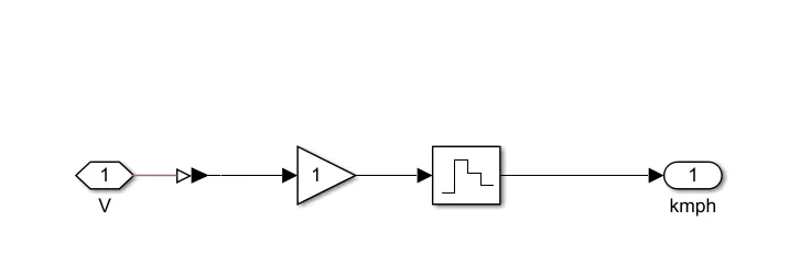
Velocity Body Subsystem-
The various blocks defined previously are connected to the vehicle body. 4 magic formula tire block are used since the vehicle has 2 axle and 2 tires on each axle. The tires are LF,LR,RF,RR. The normal port on each tire are connected to the appropriate NR and NF ports on the vehicle block. The hubs of each tire are connected together and an extra connection is made from them to the vehicle body block. The hubs of each tires are connected together and an extra connection is been made from them to the vehicle body block. the simple gear and inertia blocks are connected to the axle port of the tires. The wind velocity and road incline are provided with a constant physical signal of 5 m/s and 0 degree respectively. The velocity port has been connected to the velocity subsystem and connections from the subsystem is open to the ‘V’ port. The base port of the simple gear has been left open to the ‘R’ port to take in a rotational signal. If all these connections are made, all of these components can be selected and made in to a subsystem.
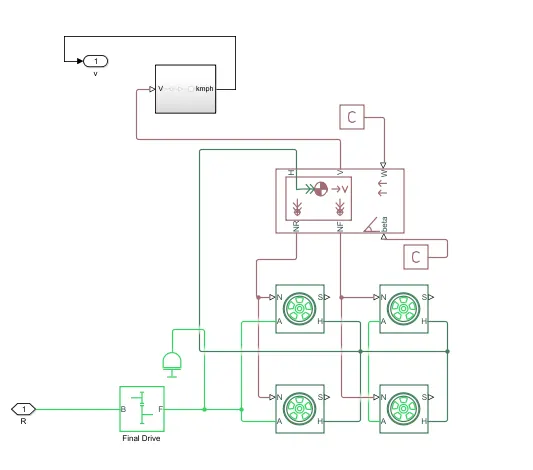
The subsystem is created so that less space is taken up in the workspace and now, we only need the open ended connection to be modified.
Motor
For the EV model we have selected to use a DC block as the motor. This is because DC motors are easier to model and have fewer parameters to modify for a particular application. For this model a dc motor will do just fine.
As we can see there are 2 sides to the block, the mechanical side on the right and electrical side on the left. The mechanical side has 2 port, C and R. The C stands for casing and R stands for rotation of the rotor producing torque. The electrical side has positive and negative terminal for the voltage to be applied.
If a positive voltage is applied to the DC motor block from the positive to the negative terminal, a positive torque will act from the C port to the R port. The direction of the torque produced by the DC motor can be changed by changing the sign of back emf or the torque constant. The C port of the mechanical side needs to be connected to a mechanical rotational reference because it will be stationary. The R port will be connected to the open connection to the open connection of the simple gear from the vehicle body block. the positive terminal on the electrical side is connected to the positive terminal of a power converter which in my case will be an H bridge.
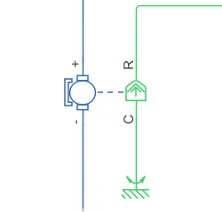
The mechanical rotational reference block is shown below.
Double clicking the DC motor block takes us to its parameter. The electrical torque parameter are first considered. Here we have chosen to parametrized the block ‘BY Rated power, rated speed rated load and the DC supply voltage which were changed to the value shown in the image.
In the mechanical parameter we can modify the rotor inertia, damping and initial rotor speed. However, these values were kept to default settings.
Once the DC block has been parametrized the following connections were made.
Power converter
The power converter is needed to provide power to the correct form and magnitude from one component to another. In this case power converter is used to provide a DC voltage from the battery of the EV to the DC motor so that it can operate properly with the required parameter. As mentioned earlier, a H bridge is used as power converter.
The H bridge has 2 sides, the left side is for controlling of the voltage signal and the right side is for the terminal to provide the controlled voltage to the DC motor. The left side port of the H-bridge block are;
PWM- This stands for Pulse Width Modulation which will provide the voltage pulse to the H-bridge either in the pwm or average mode.
REF- this stands for Rference
Rev- Stands for reverse
BRk- this stands for Brake
Opening the H bridge the parameter window will popup. The main parameter are the simulation model and load assumptions of the H bridge. We have selected the H bridge to run on an internal power supply with an averaged simulation mode instead of PWM mode. This is because using PWM mode will result in significantly longer simulation time compared to using the averaged mode. Regenerative braking mode is enabled and the current characteristic to the smoothed option.
The next parameter of the H bridge are input thresholds. Here we can set the various voltage limits of its 4 left hand side ports. These values are left to their default settings.
The last parameter for the H bridge pertain to its bridge parameter. Only the first parameter of output voltage amplitude was modified. This is because the DC motor has been parametrized to run on a DC supply voltage of 330V. So this same value is used for the output voltage amplitude.
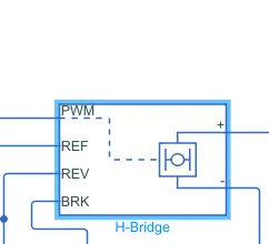
Once these parameters are set the connections to the blocks are made.
Controlled PWM voltage
In the next step a Controlled PWM block is been used to provide a controlled pulse width modulated voltage to the H-bridge block.
The block will output the PWM voltage through its PWM and REF ports which will feed in to the same port found on the H-bridge block. if the pulse is low the output voltage is considered 0V whereas if the pulse is high the output voltage will which is set to 330V in the H bridge block. the pulse of voltage created by the block are dependent on the duty cycle which is the radio of the time that the switch is ON to time taken for 1 cycle. The duty cycle is set by the input of the controlled PWM voltage block.
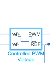
The duty cycle formula is given by:
The block parameter are shown in the image
The main setting pertains to the PWM parameters. Here all the parameter are maintained at their default values. I have chosen the ‘Averaged’ Simulation mode so that the average value of the voltage pulses are generated and fed in to the H-bridge. This will allow for quicker simulation times, just like for the H bridge block parameters. The remaining parameter of input scaling and output voltage are unchanged.
If these parameters have been applied, close the block parameter window. The connection for this bock will be made later on.
Controlled voltage source
The input port of the controlled PWM voltage block are still unconnected as they require a controlled voltage source to provide the voltage to produced voltage pulses to be fed in the H bridge. Thus a controlled voltage source block is been used. The block is useful to provide voltage powerful enough to maintain the voltage at the output regardless of the current that pass through it.
Two controlled voltatge sources are used in this model. One block is used to provide the voltage for acceleration of the vehicle and the other is to provide the voltage for the deceleration of the vehicle.
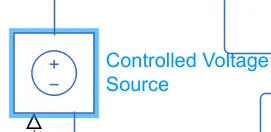
Electrical Reference.
The electrical reference block is used to create a grounding effect for electrical circuits. Any model that uses electrical or electronics component will need to have at least one electrical reference block in it.
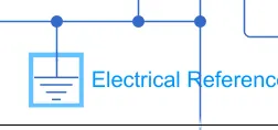
In this model, we are using this block for 2 occasions. The first is to create an electrical ground between the controlled voltage source, controlled PWM voltage and the H-bridge blocks. The second is for the battery system which will be modified afterward.
Solver Configuration
The solver configuration block is used to solve any necessary equation in a model and in my case, I have used them in the connection to the REV port of the H bridge block.
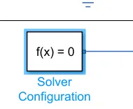
Longitudinal Driver
The longitudinal driver block is used for giving normalized acceleration and deceleration commands to a controller based on a sets of data. The first data set is a reference velocity and the second data set is the feedback velocity.
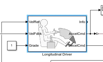
The longitudinal driver block as the following ports:
VelRef: Stands for the reference velocity and it is the velocity data provided from the drive cyclesource.
VelFdbk: stands for feedback velocity and it is the velocity data provided from the vehicle bodys velocity port outputting velocity data.
Grade: stands for grade or inclination angle for the surface on which the vehicle is travelling in degrees.
Info- this stands for bus signal which stands consisting of block calculation eg; acceleration/deceleration command.
AccelCmd : this port provides acceleration command to a controlled voltage source.
DecelCmd- this port provides deceleration command to another controlled voltage source.
The working of the longitudinal driver block is simple. The reference velocity data coming from the drive cycle source is compared to the feedback velocity data coming from the vehicle body block. if the reference velocity is lesser than the feedback velocity a deceleration command is given as the output to another controlled voltage source. For acceleration and deceleration commands are given as output signals thus we have used a PS Simulink converter block. this block is used to connect input signal to physical signal.
PI controller is used and the unit is set to m/s.
Grade
The grade port of the longitudinal driver block is connected to a constant block with a valur of 0. This is so since no road inclination is modelled for simulation.
Drive cycle
A driving cycle is a series of data points representing the speed of a vehicle versus time.
Driving cycles are produced by different countries and organizations to assess the performance of vehicles in various ways, as for instance fuel consumption, electric vehicle autonomy and polluting emissions.
Fuel consumption and emission tests are performed on chassis dynamometers. Tailpipe emissions are collected and measured to indicate the performance of the vehicle.
In this EV model a drive cycle is used as the reference velocity data for longitudinal driver block to send acceleration or deceleration commands according to drive cycle. One method is to create a drive cycle with spreadsheet of velocity data in one column and time on the second column. Another method is to use signal builder block and create signal that represent the velocities at which the vehicle should travel and duration for which those velocities are to be maintained. The last method is to use the industry standard cycles which are in built Simulink library.
By default the drive cycle block is set to FTP75 drive cycle. This can be modified by opening the block parameter.
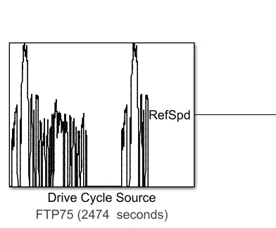
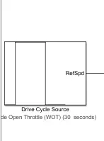
Once the drive cycle block is set the output port of the drive cycle can be connected to the reference speed port of the longitudinal driver block. If all the parameters have been set as discussed the connections can be made.
The connection for the vehicle feedback is left open ended for now and will be connected later on. Next we can model the battery of the EV
Battery System
The battery is the energy store of the EV and will contain the electrical energy in DC form and provide this energy to the DC motor for it to operate. The battery block used is a simple one and consider only the basic parameter.

As we can see the battery block parameter includes the nominal voltage the internal resistance and the battery charge capacity. We have used a nominal voltage of 440V and internal resistance of 0.2 ohms and an infinite battery charge capacity. The nominal voltage is selected so that it is more than sufficient to supply the voltage to the DC motor and the H bridge block.
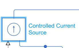
Current controlled source
The controlled current source block is a part of the battery system used in E model. Similar to the controlled voltage source this block will represent an ideal current source that is powerful enough to maintain the specific current regardless of the voltage across it.
Current sensor
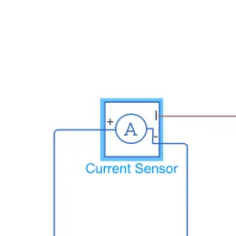
The Current Sensor block represents an ideal current sensor, that is, a device that converts current measured in any electrical branch into a physical signal proportional to the current. The block is used to measure current between battery circuit and DC motor.
The positive and negative terminal represent the terminals across which the current sensor is inserted in to the circuit. The third port outputs the physical signal and in this model it will send signal to the controlled current source.
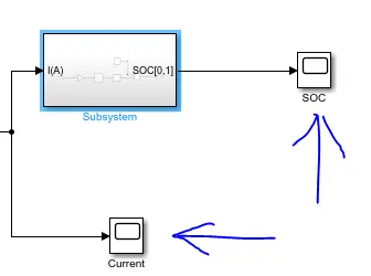
SOC and current
SOC stand for state of charge and it is a measure of the available charge in a battery. When the battery is fully charged it is considered as 100% charged and 0% if completely discharged. In the EV model we want to measure the current and the SOC of the battery as the simulation is run. For this we have used a scope block which shows the output signal we wish to measure in the form of a graph plot. 2 scopes are used in this EV model, one for the current and the other for the SOC. In order to measure it a PS Simulink converter is to be used.
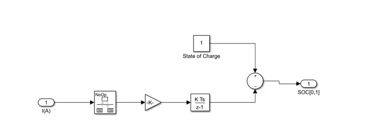
SOC Subsystem
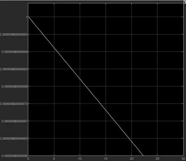
To measure the state of charge of the battery a subsystem was created of various blocks. The first block is the rate transition block used to handle transfer data between different rates and tasks. Next a gain block is used to multiply or divide the signal incoming from rate transition block. in this case the gain block will divide the current signal with ampere rating of battery which has been taken as 80Ah multiplied by 3600. Then a discrete time integrator block is used to perform a discrete integration of current signal with respect to time. A constant block is used to represent the initial SOC of the battery. Assuming that the battery is always fully charged when performing the simulation. Next, is the sum block used to perform addition and subtraction operations. The signal from discrete-time integration block will be subtracted from the constant block representing 100% charge.
These blocks are then made in to a subsystem called SOC Estimate and linked with battery circuit using PS Simulink Converter block to plot the output signal of the current from the battery. Another scope is used to plot the output signal of SOC from the SOC subsystem.
Speed Measurement
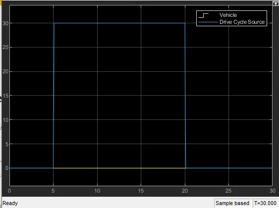
The speed measurement in the EV model is done by using a scope block modified to have 2 input port. One port takes output velocity from the vehicle subsystem block and the other takes output signal from the reference velocity port on the longitudinal driver block.

Distance measurement.
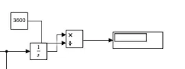
We have a scope block and a mathematical operator block to measure the distance travelled by the vehicle according to the drive cycle data. The area under the velocity time graph tells us the distance travelled by an object and so in my model. This means that the integral of the velocity with respect to time, gives us the distance travelled. Thus we have implemented the integrator block to integrate the velocity signal that is output from vehicle subsystem.
From the integrator block we need a divide block along with constant block having the value of 3600 in order to convert the divide the integrated speed signal which is in kilometer per hour by 3600
Finally a Display block is used to show the distance traveled as the simulation runs.
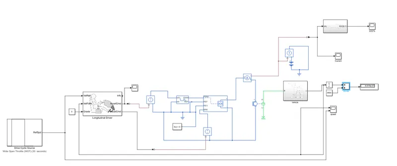
After all the connections are made, we can run the simulation.
Results
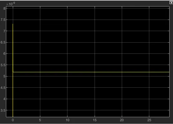
We ran the WOT drive cycle and took the output given for speed current and SOC Scopes. The distance traveled by the vehicle in the drive cycle was also measured using a display block. the stop time was set to 30 seconds before running the simulation
Current Measurement
SOC Measurement
Speed
Conclusions: -
The EV model has been created with necessary block components using Simulink software and model has been simulated for a customized WOT duty cycle. The simulation has produced results of the velocity of the vehicle, a current flowing from the battery as well as the distance traveled by the EV. Since the EV model was parameterized to simulate averaged voltage pulses in the H bridge and controlled PWM voltage blocks to be fed into DC motor, the simulation was fast. The EV model was able to follow the commands given by the reference velocity from the given duty cycle. The discrepancy between the reference velocity and the actual velocity can be attributed to a variety of factors including vehicle inertia, transmission inertia, transmission system.