Final Project: Design of an Electric Vehicle

AIM

Create a MATLAB model of an electric car that uses a lithium-ion battery and induction motor. Choose suitable blocks from the Powertrain block set. Prepare a report about your model including the following:

1. System-level configurations

2. Model parameters

3. Results

4. Conclusion

Introduction

Electric Vehicle paved their way into public uses as early as the middle of the 19th century, even before the introduction of gasoline-powered vehicles. In the year 1900, 4200 automobiles were sold, out of which 40% were steam-powered, 38% were electric vehicles and 22% were gasoline-powered. However, the invention of the stator motor, improvement of mass production of gasoline-powered vehicles, and inconvenience in battery charging lead to the disappearance of EV in early 1990.

However, in recent, environmental issues and unpleasant dependence on oil led to the resurgence of interest in Electric Vehicles. Interest and research in EV's soared in the 1990s with the major automobile manufacturers embarking on plans for introducing their own electric or hybrid vehicles. The top-level perspective of Electric vehicle is shown below:

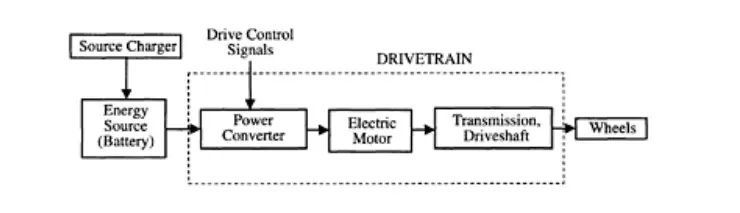
• The trend increases today, with Electric vehicle serving as zero-emission vehicles and hybrid electric vehicles already filling in for ultralow - emission vehicles.

EV is simpler than an HEV. Its basic system‐level constituents are shown below:

• The complete EV consists of not only the electric drive and power electronics for propulsion, but also other subsystems to make the whole system work.
• We need a battery (or a fuel cell) to provide the electrical energy. This is shown by the block on the left, which provides the power to drive the electric motor. The motor is part of the EV powertrain, labeled as EVPT on the right. For each of these items, battery, or EVPT, there is a controller.
• The battery controller controls the charging or discharging, and similarly, the EVPT controller controls the speed or torque of the motor by controlling the power electronics.
• The position of these items is subtle design issues involving cost and packaging. In addition, there is a box shown as the interface. This is the controller box that receives signals and also power, both high voltage for propulsion and low voltage for certain specific devices that operate at low voltage, and then through the interface function channels them to the EVPT motor or the high‐voltage battery. Again, these functionally separate blocks may be merged when physically integrating the system.
• In addition to the above blocks, there are various other blocks, for example, the vehicle controller, which can receive signals such as the velocity of the vehicle, and driver pedal position, and make a decision whether or not additional torque is needed from the motor. Based on that information it can send a signal to the EVPT controller with the appropriate torque request.
• Similarly, the brake controller can receive signals corresponding to brake pedal position, vehicle velocity, and so on, and decide how much brake force is needed. It can also receive signals such as the battery’s state of charge and figure out whether the opportunity of regenerative braking is present. If so, it can then send signals to the EVPT controller to carry this out.
• Information transmission between various blocks is normally done through a controller area network (CAN) bus. This is basically a type of computer network where a single wire (which could also be a twisted pair of wires) can contain a variety of information or communication signals multiplexed together. Some sort of protocol has to be observed when multiple signals are passed through and shared by a common medium.

----------------------------------------------------------------------------------------------------------------------------------

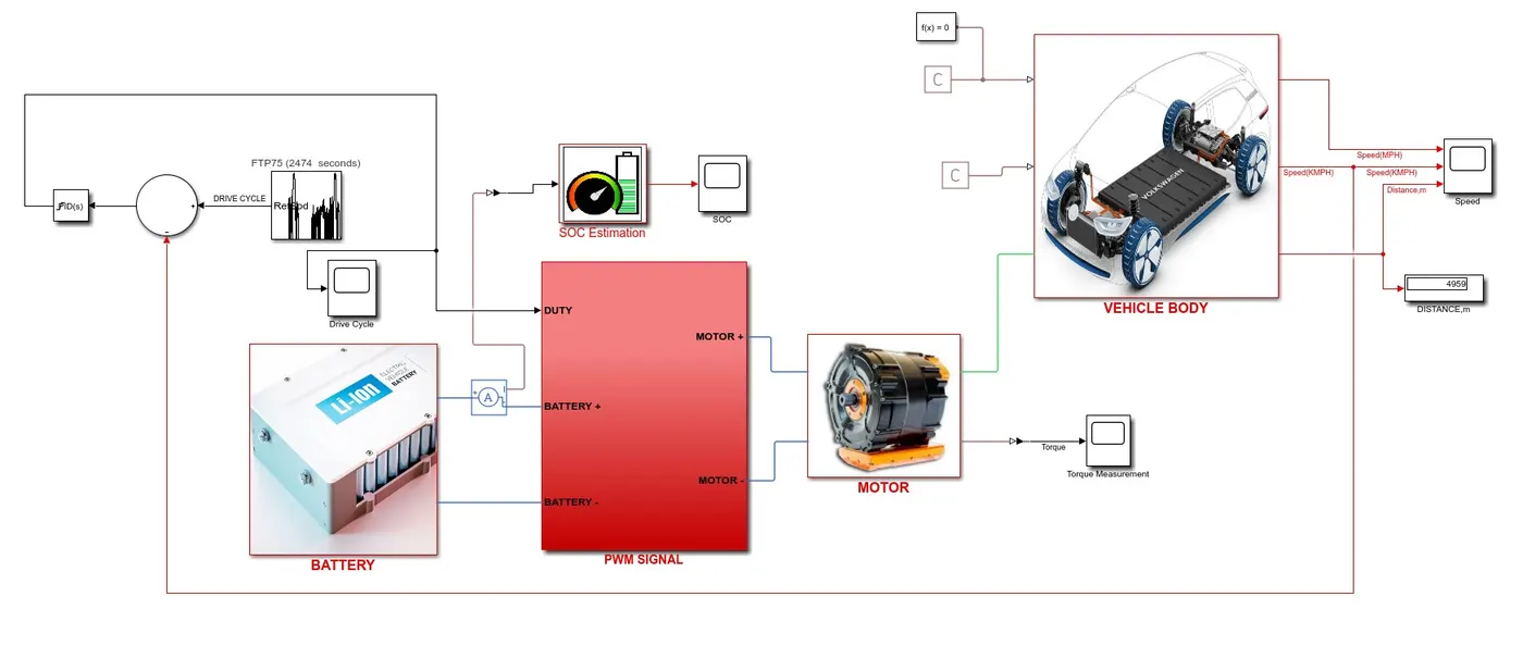
SIMULINK MODEL DESIGN

• For our project design of vehicle consists of the design of vehicles at various subsystems:
• Design of Vehicle body, which consists of our physical vehicle parameters which are implemented here.
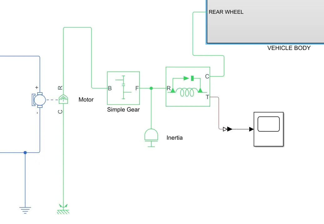
• The vehicle body is controlled by the Motor, which is connected to the axle of the rear vehicle with the gear system.
• Motor torque is controlled with the PWM(Pulse width modulation) signal to which the battery signal is supplied.
• Our model is backward-facing model and it is closed-loop, start with the tractive effort required at the wheels, and “work backward” toward the engine.

Various Parameters which are considered in our design are:

Mass of Vehicle(passenger mass included) = 1080 Kg

Frontal Area of Vehicle, = 1.33 `m^2`

Drag Coefficient = 1.2

The radius of Wheel = 18 in

Rolling Resistance COefficient = 0.005

Cell Voltage = 5 V, consists of 96 cells connected in series and parallel

Components

Vehicle Body :

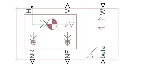
The Vehicle body represents a two-axle vehicle body in longitudinal motion. The Vehicle can have the same or a different number of the wheel on each axle. For example, two wheels on the front axle and wheel on the rear axle. The vehicle wheel is assumed identical in size. The vehicle can also have a center of gravity(CG) that is below the plane of travel.

The block accounts for body mass, aerodynamics force, road incline, and weight distribution between axle due to acceleration and road profile. The vehicle does not move vertically relative to the ground.

INPUT

W: It signifies the signal port for headwind speed.

Beta: Input from this port is the road inclination angle.

OUTPUT

V: The output from this port is vehicle longitudinal velocity in m/s.

NF: It gives the output for normal force on the front axle. Wheel force is considered positive if acting downwards.

NR: It uses to connect the rear wheel with the vehicle body. It gives the signal output port for normal force on the rear axle.

H: It uses to provide a mechanical translation. It is associated with the horizontal motion of the vehicle body.

Parameters

The parameters provided for this vehicle body is shown below:

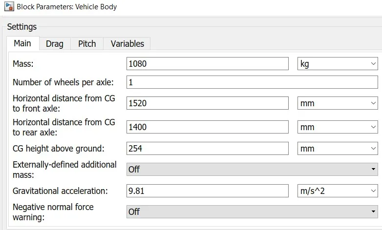
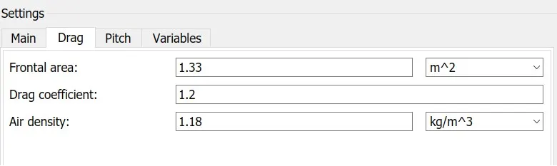
Some of the parameters is shown above, with mass to be 1080 kg, center of gravity to be 254 mm. Drag coefficient and frontal area to be 1.2 and 1.22m^2.

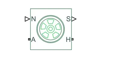
Tire(Magic Formula):

This blocks model a tire with longitudinal behavior given by the magic formula, which is an empirical equation based on the four fitting coefficients. The block can model tire dynamics under constant or variable pavement conditions.

The tire block model the tire as a rigid wheel-tire combination in contact with the road and subject to slip. When torque is applied to the wheel axle, the tire pushes on the ground and transfer the resulting reaction as a force back on the wheel. The action pushed the wheel forward or backward.

The tire block is shown below:

INPUT

N: It is associated with a normal force acting on the tire. The normal force is positive if it acts downward on the tire, pressing it against the pavement. It is used to connect with the body parts.

A: It is a mechanical rotation port, it is associated with the axle of the tire.

H: It is a mechanical translational port associated with the wheel hub that transmits the thrust generated by the tire to the remainder of the vehicle.

OUTPUT

S: This port is associated with the relative slip between the tire and the road.

Parameters

The parameters for a tire is given below:

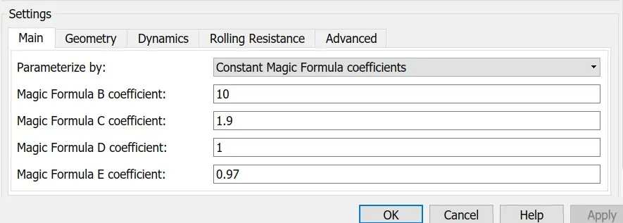
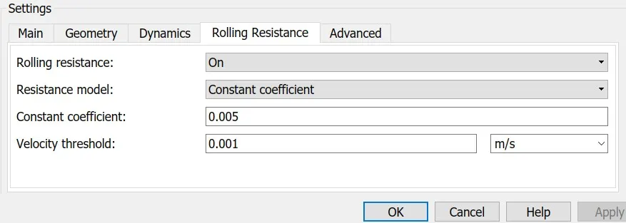
The tire is modeled with the above characteristics with the radius of the tire to be 18 in and the inertia of the tire has also been modeled. Rolling resistance has also been considered for the tire.

After that connection of the tire with the vehicle, the body has been made for the Vehicle subsystem, Which is shown below.

The vehicle subsystem model consists of various sensors, to plot the longitudinal force, the normal force of tire.

Ideal Force Sensor

The ideal force sensor is used to calculate the longitudinal tire force of the tire. It is connected with the hub port of the tire, which converts the PS Simulink converter to convert the signal to the plot.

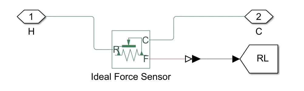
Normal Tire force is also plotted for the system for both the real and front wheel.

So the main system of the model is shown below:

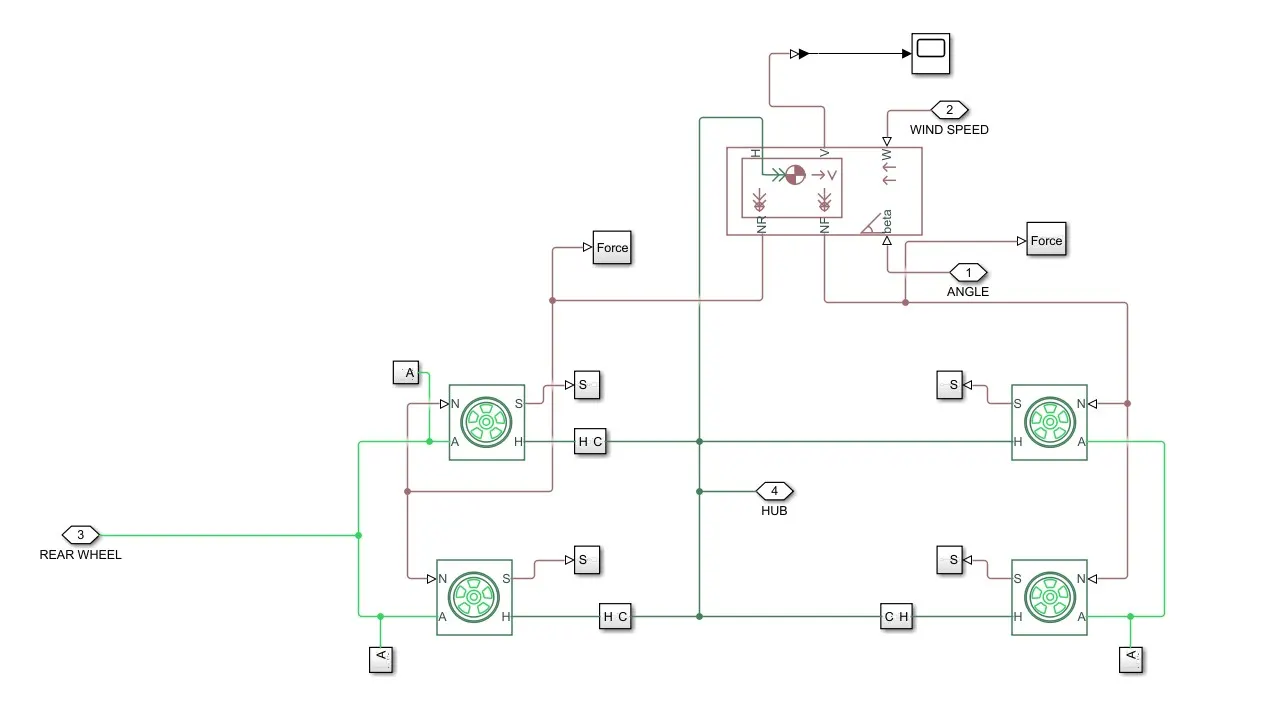
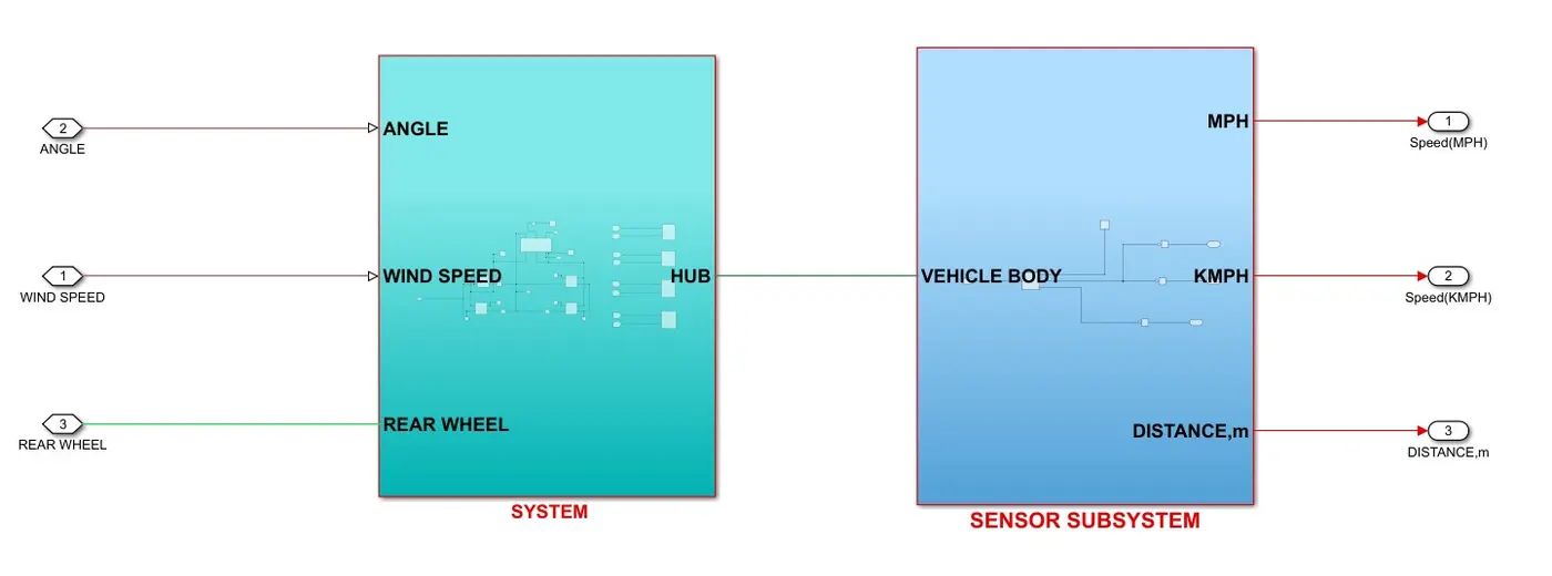
This is put into a subsystem, which is connected with the sensor subsystem to model the velocity output and distance covered by the system.

The sensor subsystem consisted of an ideal translational motion sensor which is connected with the hub of the vehicle to measure velocity and distance covered by the vehicle.

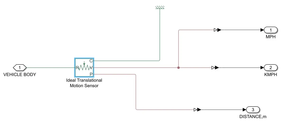
So finally the vehicle body subsystem consists of the main body and sensor system, which is shown below:

Simple Gear

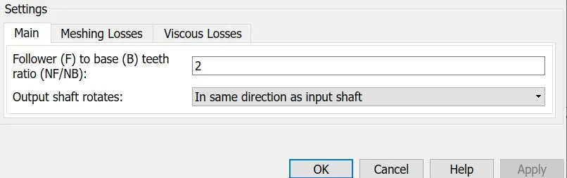
Simple gear is used which is connected to the rear wheel axle. It represents a gearbox that constraints the connected driveline axels of base gear, B, and the follower gear F, to corotate with a fixed ratio.

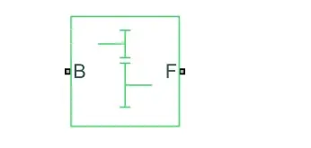
INPUT

B: It represents the rotational mechanism associated with the base or input shaft.

OUTPUT

F: It represents the rotational mechanism associated with the output shaft.

Parameters

The parameter associated with the simple gear is shown below:

MOTOR

DC motor model block is used to provide the required torque to the vehicle subsystem through the gear connection.

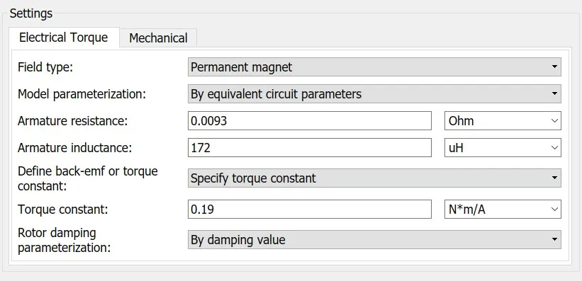
For our system, we have set the model parameterization parameter to by equivalent circuit parameters.

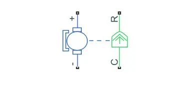
PORTS

+, Positive terminal: This port is associated with the DC motor positive terminal.

-, Negative Terminal: This port is associated with the DC motor negative terminal.

C: Mechanical rotation conserving port associated with the DC motor case. It is connected with mechanical rotational referenced.

R: This mechanical rotation port is associated with the dc motor rotor. It is connected with the simple gear in our model, which issued to supply the required torque.

Parameters

The various parameters of the motor are given below:

The motor with gear part is shown below:

PWM(Pulse Width Modulation) Average Subsystem

The pulse width modulation block is used to control the motor torque, with the duty cycle given to it. It works in accordance with the battery input which input is controlled with the controller.

A duty cycle or power cycle is the fraction of one period in which a signal or system is active. The duty cycle is commonly expressed as a percentage or a ratio. Its value range from 0 to 12.

The voltage sensor is used to measure the battery voltage and this voltage is multiplied with the duty cycle to get the supply voltage of the motor.

A controlled voltage source block is used to maintain specific voltage towards motor control.

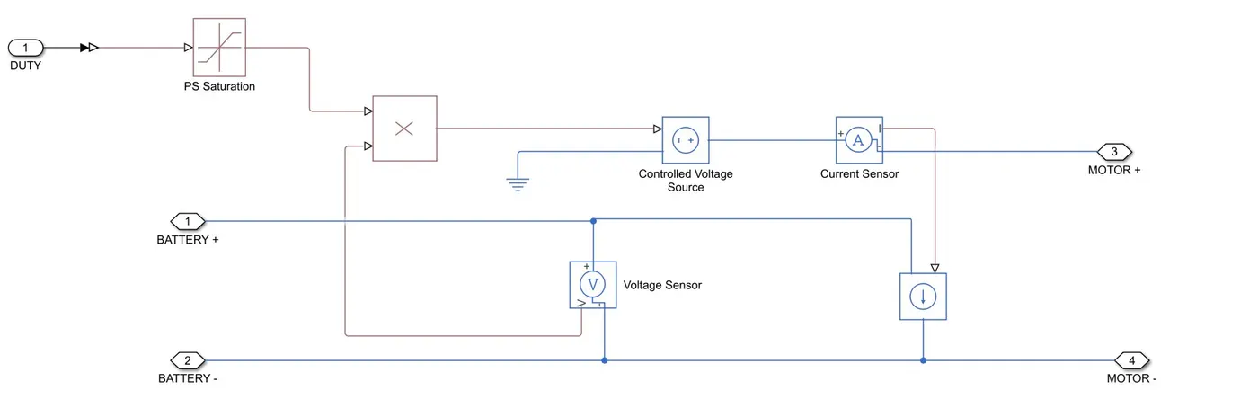
BATTERY

The battery is modeled with the help of an equivalent circuit of cell.

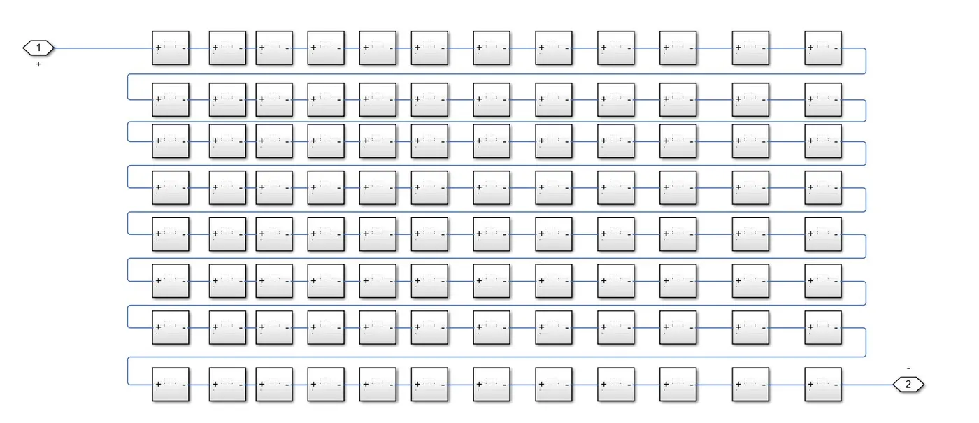
Cells are connected in parallel and series connection to form a battery pack.

The equivalent circuit of the cell is given below:

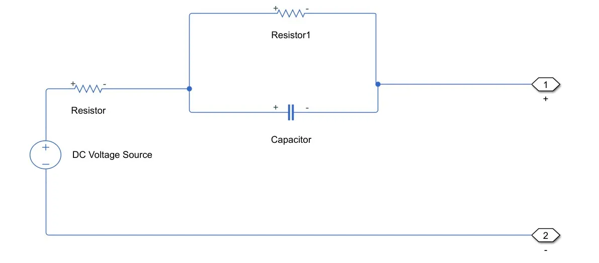
DC voltage is taken 5 V and a resistor of both systems are taken as 0.01 ohm and 0.005 ohms.

The below figure shown the collection of cells in series and parallel.

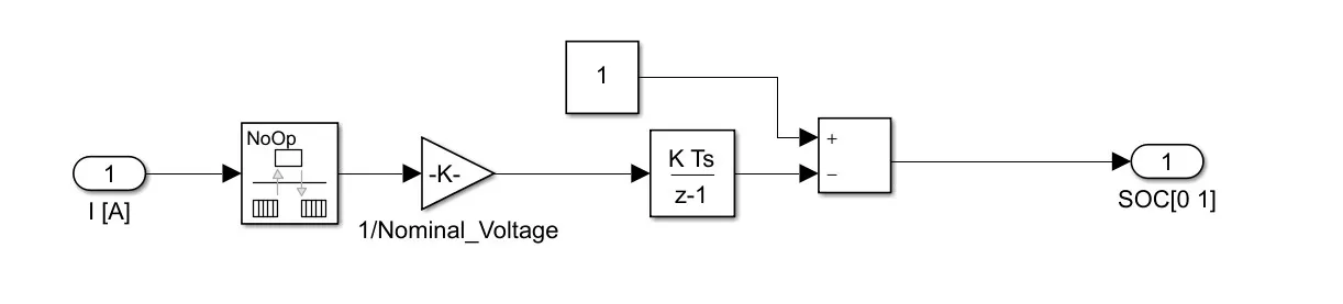
SOC calculation has also been made to know the level of batteries charge remain in the system for functioning, and when to start the regenerative braking.

Drive Cycle

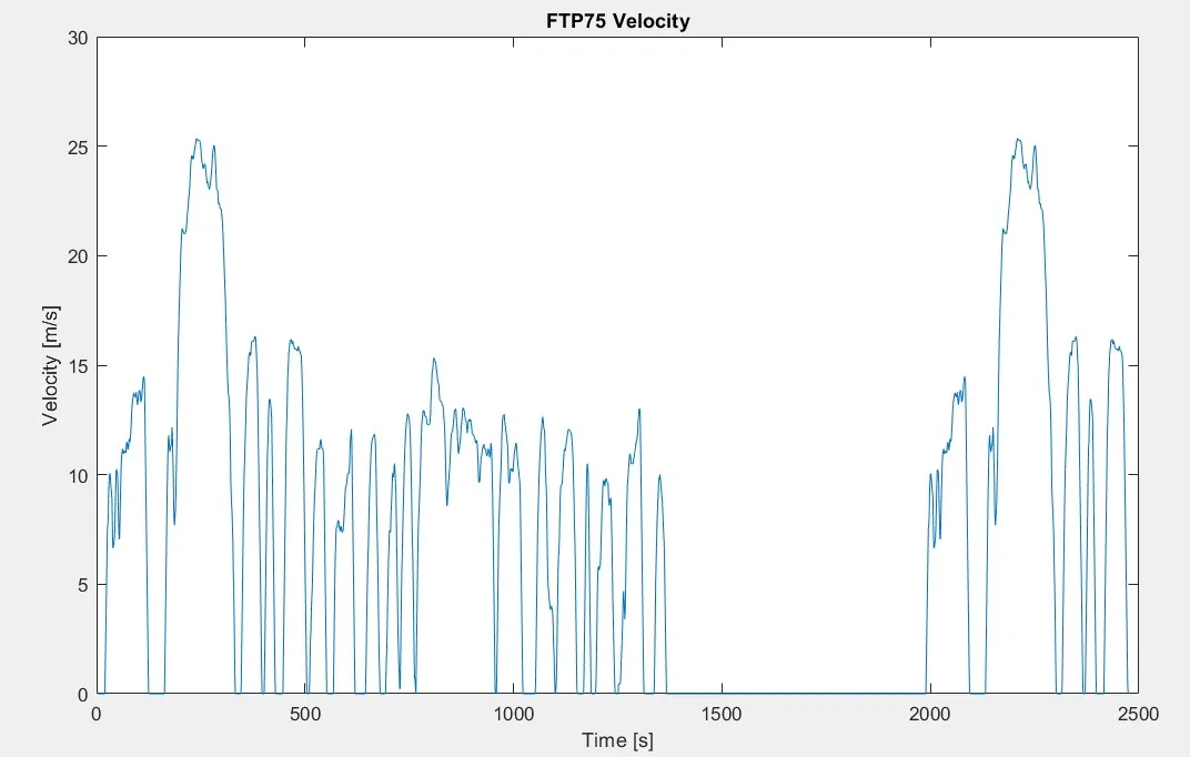
• FTP-75 drive cycle has been used for our simulation with PID controller closed loop, to get the desired drive cycle at the output.
• The FTP-75 (Federal Test Procedure) has been used for emission certification and fuel economy testing of light-duty vehicles in the United State.
• The Drive cycle is connected to the Duty cycle block of the PWM block.

So, the complete model of our system is shown below:

OUTPUT

CASE 1 : FTP75 Drive Cycle

Our Simulation consists of FTP75 drive cycles as our reference speed which is compared with our output speed to get the desired speed with the help of the PID controller.

Vehicle Speed comparison with the reference drive cycle is shown below:

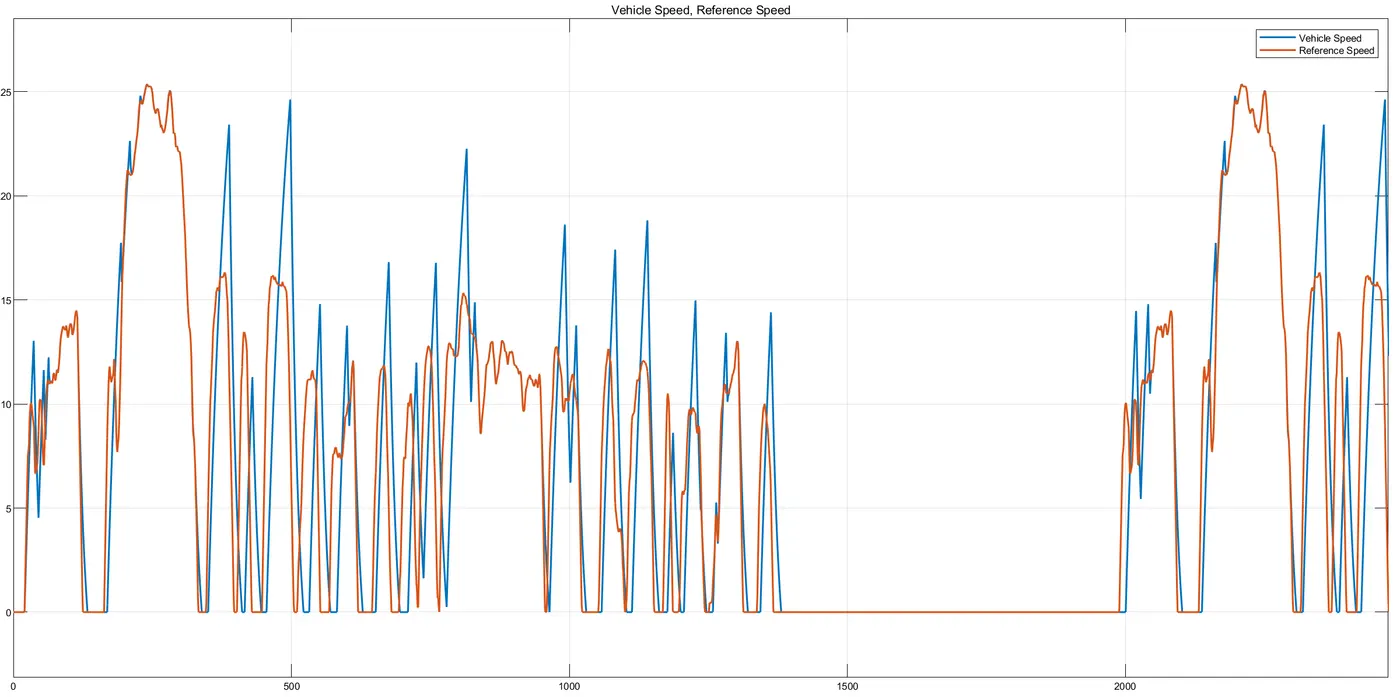
Here, the blue line refers to the output vehicle speed and the orange line refers to the reference drive cycle. The small fluctuation in the result is due to the shoot of the PID controller which is used here. This can be improved by the use of H- bridge or class E-chopper for better accuracy.

Duty Cycle Plot

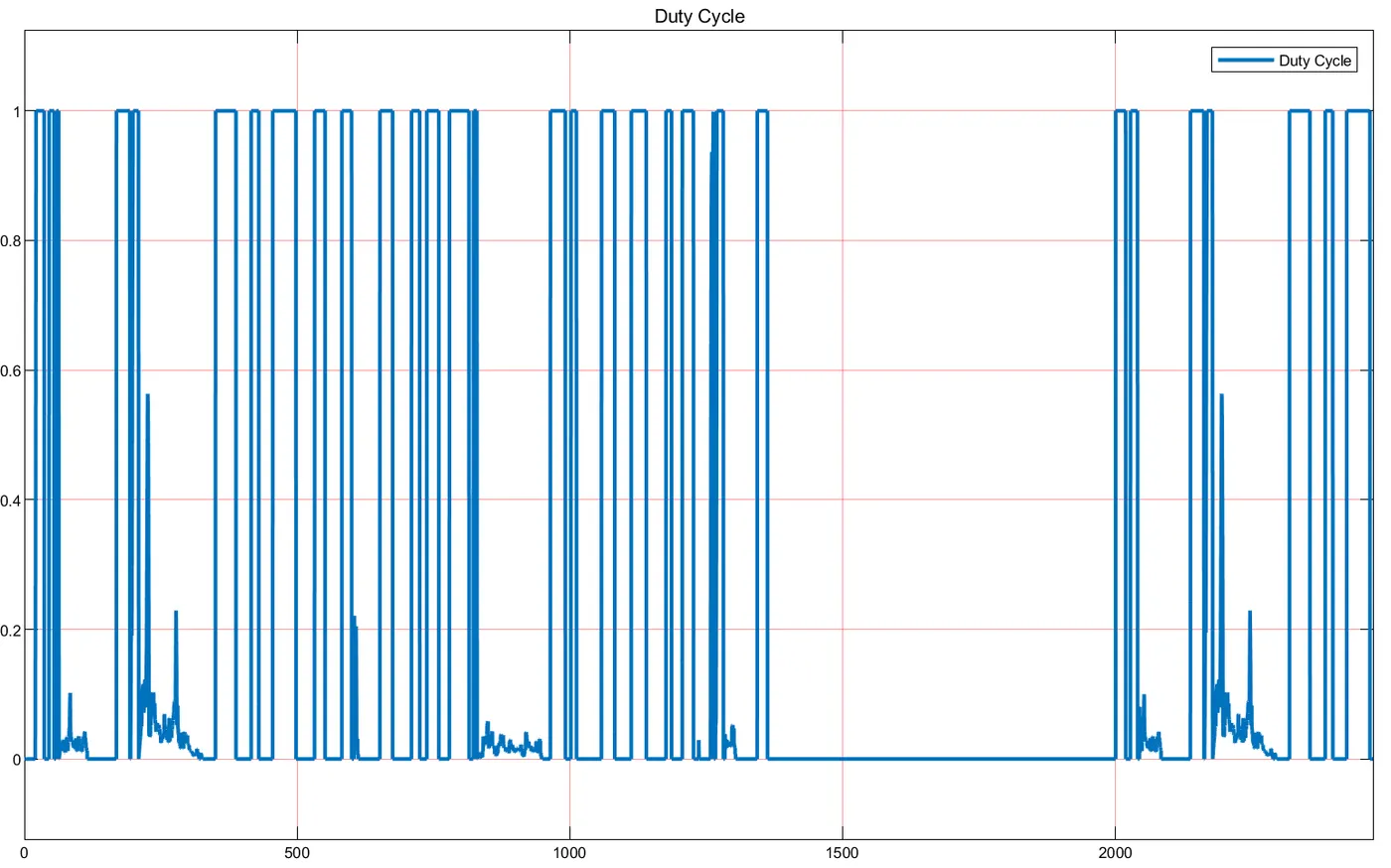
The given plot showed the duty cycle of the vehicle. We can see that at the beginning the duty cycle is zero as the vehicle has zero speed at the beginning.

After a few second the vehicle speed changes to maximum which is indicated by the duty cycle 1, which allow the full rated power use of DC motor.

Again the change in the duty cycle is represented by the use of the PID controller which tries to maintain the desired drive cycle speed at the output as at input.

I can see that there is a stop in the vehicle speed it is because of the drive cycle we are using it is indicated by the 0 here.

Vehicle Speed and Distance Covered

The given plot shows the vehicle speed of the rear and front tire and the distance covered by the vehicle during simulation.

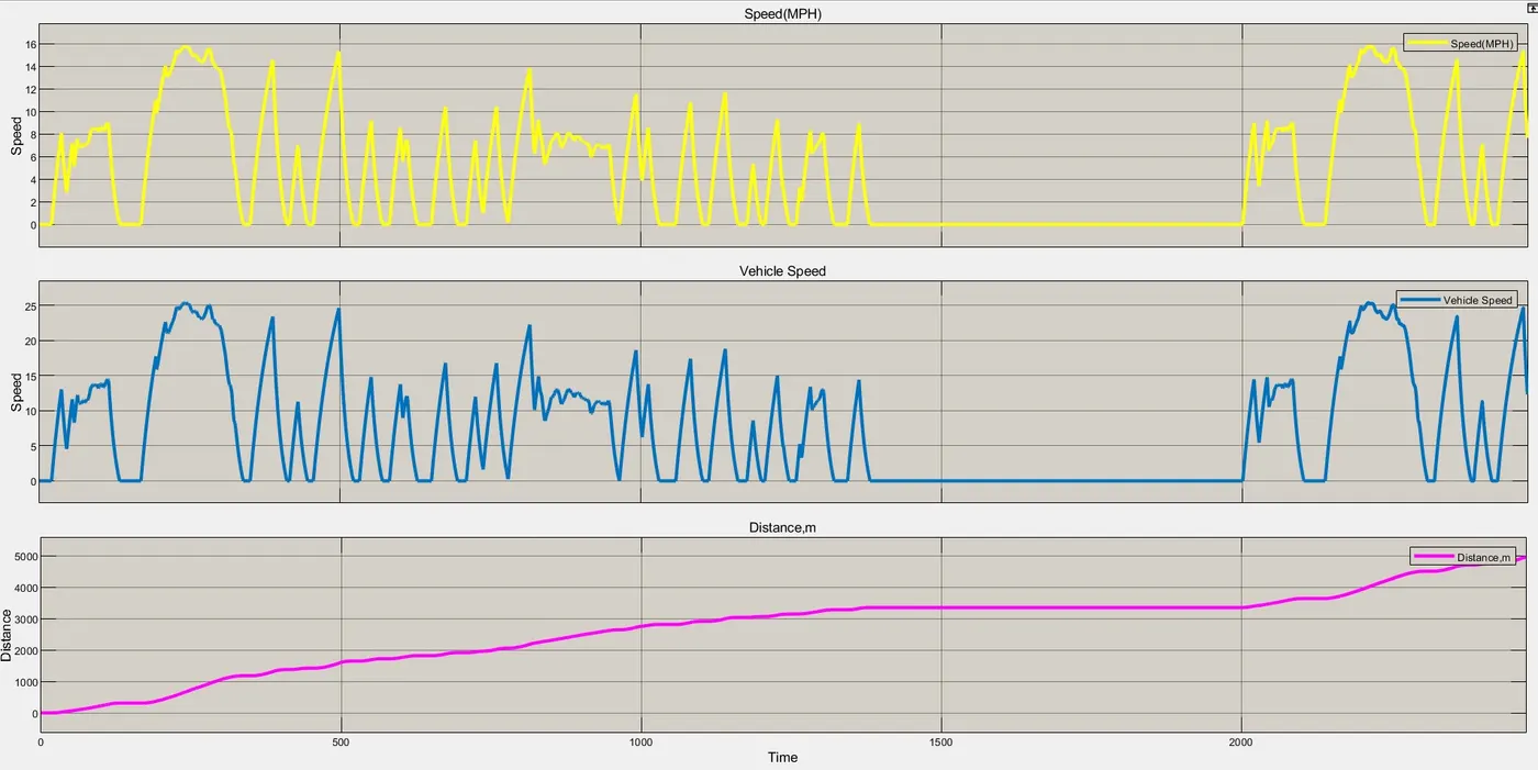
The total distance covered by the vehicle is 4959m which is 4.9 Km during the run time of the vehicle simulation.

Longitudinal Tire Force

Longitudinal tire force of the tire for the front and rear vehicle is shown below.

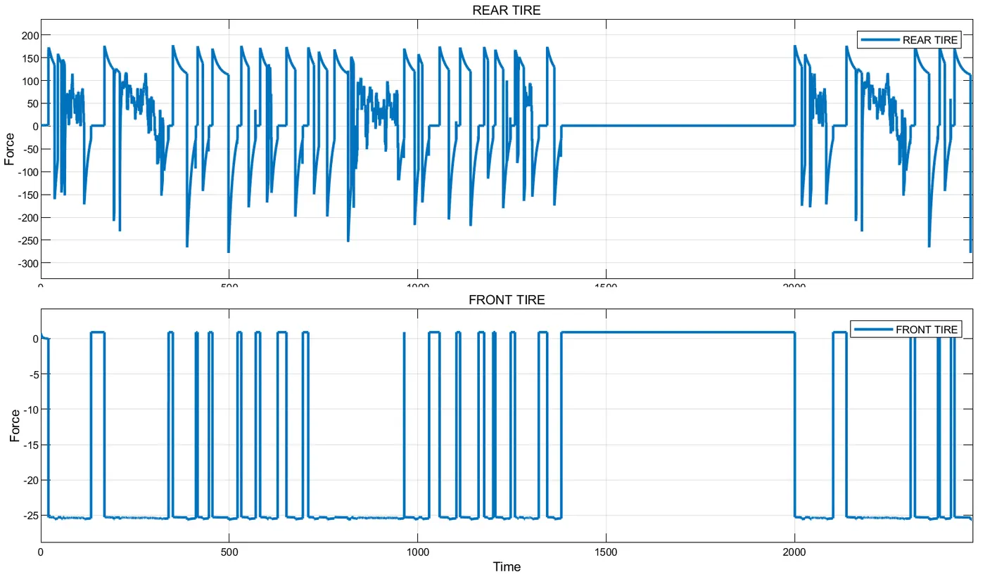
The given plot shows the longitudinal force generated by the tire which pushes the vehicle forward . As the vehicle is rear-wheel driven, we can see more fluctuation by that tire and more force is generated by that tire as compared to the front wheel.

Normal Tire Force

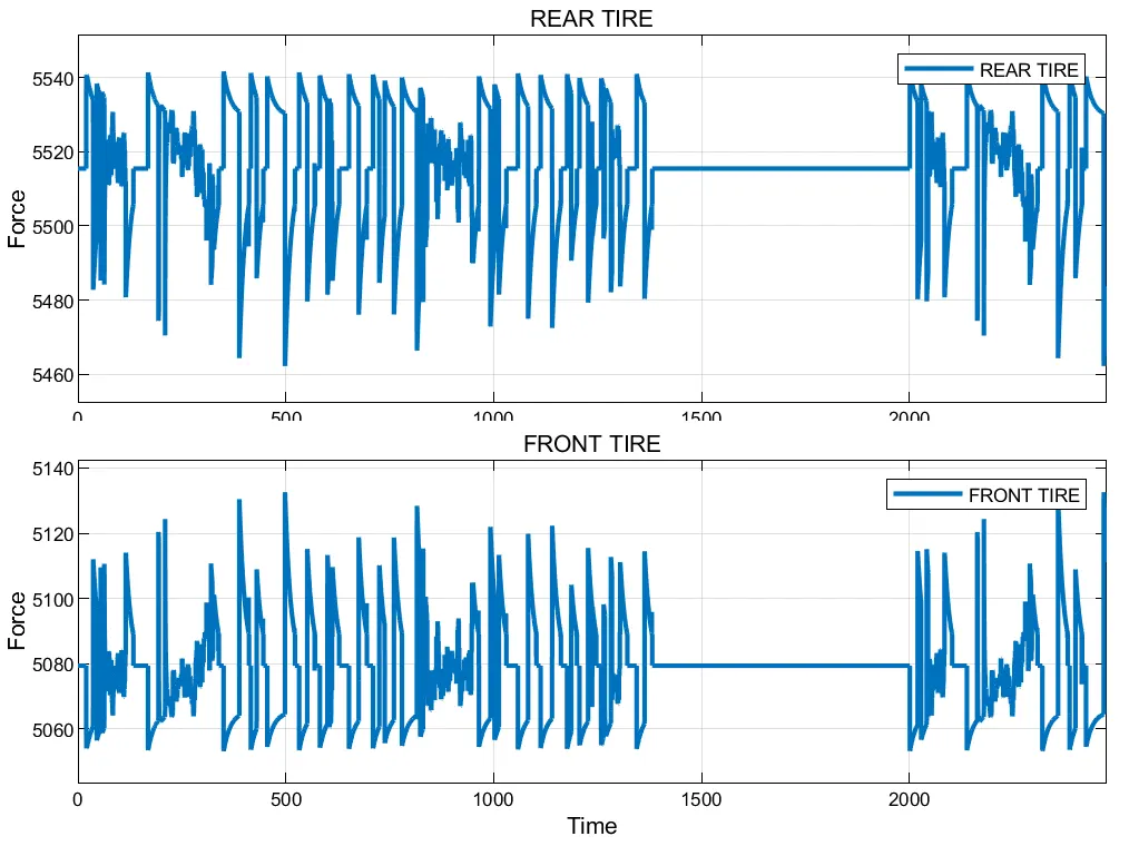
From the above plot, we can see that the normal force on both the front and rear is almost the same. As the vehicle starts to accelerate, the weight is transferred to the rear wheel as it is rear-wheel drive, so the normal force on the rear wheel increases and weight on the front-wheel decreases.

CASE 2 : WOT (Wide Open Throttle) drive Cycle

Drive Cycle

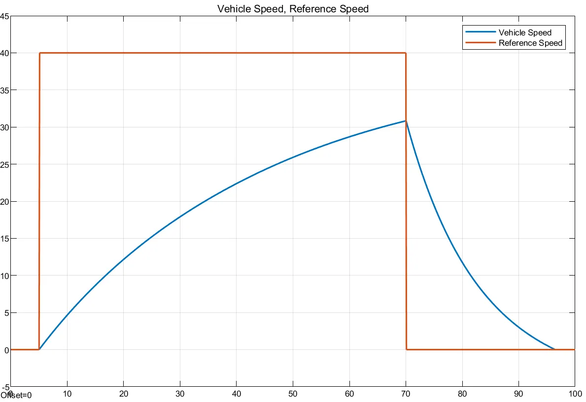
Vehicle speed doesn't follow much the given drive cycle as input but we can see that there is a declearation after the given time.

Further improvement can bbe ddone to match the input drive cycle by tuning the PID cycle further as per requirement.

Torque Output of Motor

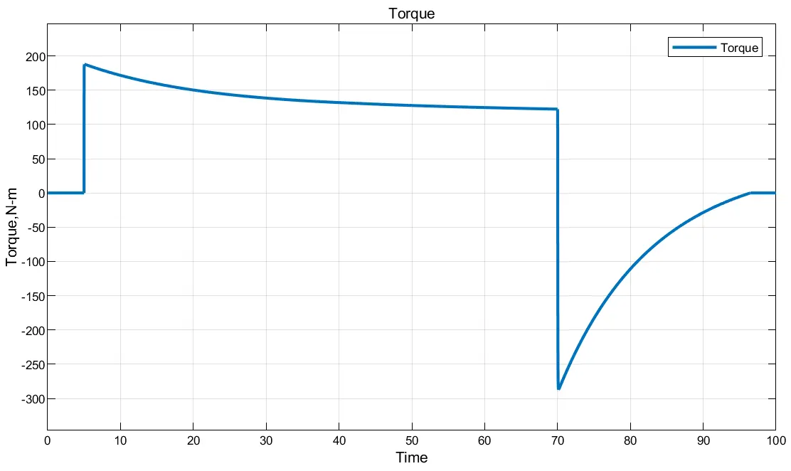
From the above plot we can se that the torque produced by the motor. At beginning we can see that the toque is zero as the vehicle is at off position . As the vehicle starts to accelerate the torque of motor also increases to maximum rated torque at maximum speed.

During decleration of vehicle , we can ses that the torque of motor decrease and become negative which can be used for regenerative braking of motor , which charge the vehicle at then then torque become zero as the vehicle stops.

SOC Estimation

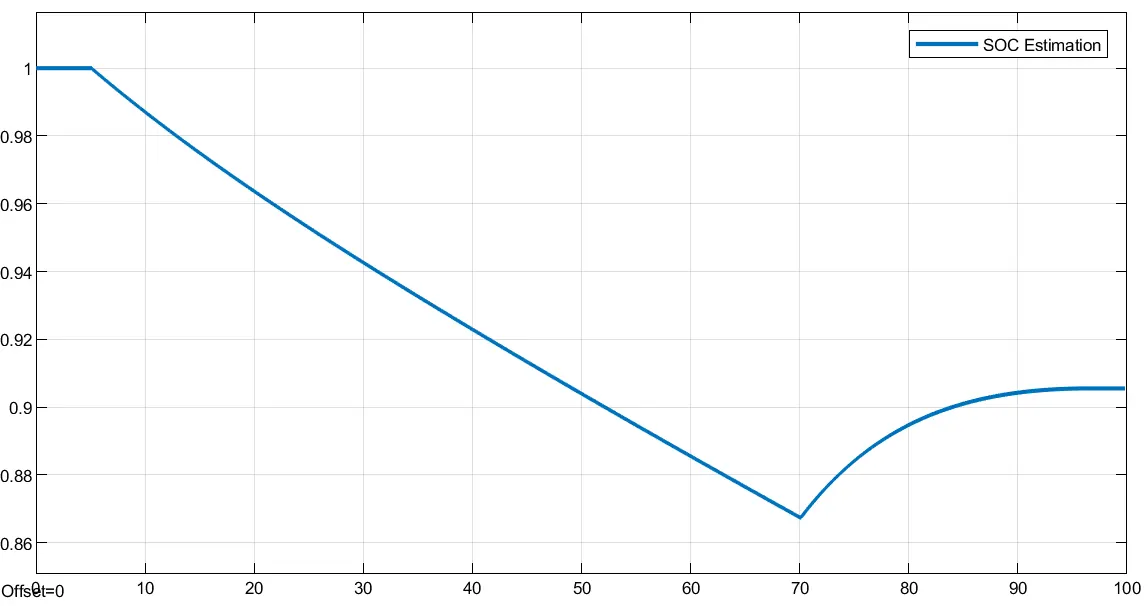
From the above plot we can see that the charge level of battery , as the vehicle starts to accelerate the battery charge level decreases and during deceleration after 70 sec during regenerative braking we can see that the SOC level of battery increase because of charging.

Vehicle Speed and distance Covered

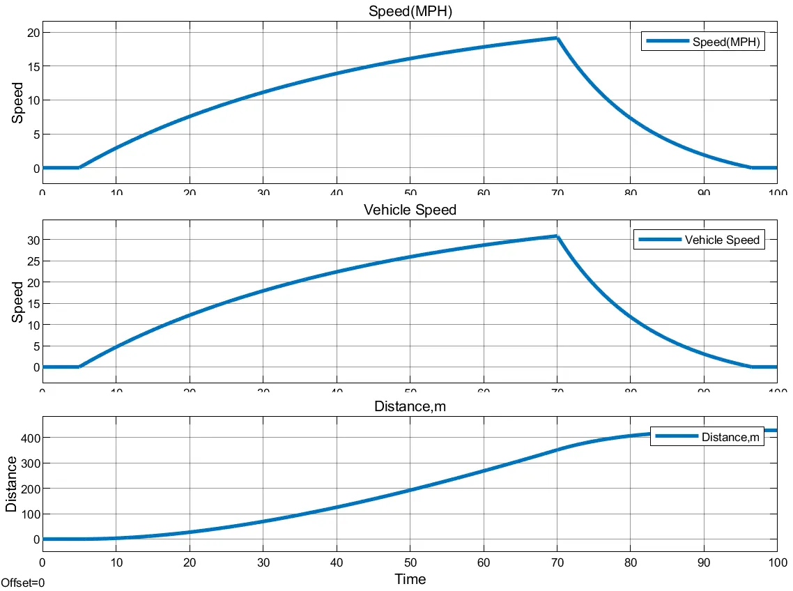
From the above plot we can see that the vehicle drive speed and drive cycle it follow. Ans we can also see distance covered by the vehicle. Totaol distance covered by the vehicle during runtime is 428.8m.

Conclusion

Pure Electric Vehicle model has been successfully designed in simulink .

Two different drive cycle is implemented and their drive cycle had benn successfully has been implemented.

Reference

1. David McDonald, Electric Vehicle Drive Simulation with MATLAB/Simulink, LSSU Sault Ste Marie, MI 4978

2. Schaltz, Erik, Electrical Vehicle Design and Simulation ,2011, Electric Vehicles- Modelling and Simulations

3. Sean Christifor McTrustry, Modelling and Control of Electric Vehicles with individuaslly actuated in wheel motors,2016,University of Wollongong Thesis Collection-1954-2016.