FINAL INDEPENDENT PROJECT

Title : To develop and compare, coulomb counting algorithm and extended kalman filter algorithm for samsung 18650 20r lithium-ion cell through DST experimental data and, To plot and regression data fit of SOC-OCV curve through low current experiment data for use in algorithm in MATLAB

Objectives :

1. To plot and regression data fit of SOC-OCV curve through low current experiment data for use in algorithm

2. To develop coulomb counting algorithm for samsung 18650 20r lithium-ion cell

3. To develop extended kalman filter algorithm for samsung 18650 20r lithium-ion cell

4. To test both the algorithms in DST cycle test experiment.

5. To compare the results for both the algorithms and study the compunding effect of measurement noise for coulomb counting in MATLAB.

Project Outline : For this project, experimental data of lithium-ion cell (which needs highly sophisticated instruments) is taken from "Centre for Advanced Life Cycle Engineering" of University of Matyland, US. They did experiments on different lithium-ion cells of different form factors. We will choose samsung 20r 18650 cylindrical type lithium-ion cell, since cylindrical cells are one of the most commonly used cells in Electric Vehicles due to their manufacturing cost (even Tesla uses cylindrical cells). Link for the data:

https://web.calce.umd.edu/batteries/data.htm

Now, first we need to compute State of Charge (SOC) by Open Circuit Voltage (OCV) curve and corresponding regression fit function so as to use in extended kalman filter algorithm. For that we will use low current data from the portal. Now, a common confusion is that why are we taking any current when we need open circuit voltage. When, current is very low, voltage across the battery is almost equivalent to open circuit voltage of battery. Because, essentially open circuit voltage is the voltage of battery without polarization and when current is very low, then polarization (represented by internal resistance in randle's battery model) is also very low. Thus, we can use low current data to calculate SOC-OCV curve. Here, low current is 0.1A and cell capacity is 2000mAh, thus it is discharged at 0.05C (way below recommended value of 0.2C for SOC-OCV curve).

After, calculating SOC-OCV curve, we will do regression fit of the data to be used in algorithm i.e. to approximate the curve with a suitable function. After, that we will input DST cycle data for the computation by the algorithms from the experimental data conducted by CALCE group. First, we will do computation by coulomb counting algorithm. Let's first undertand the algorithm.

Coulomb Counting Algorithm : As the name suggests, we are counting the number of coulombs entering or leaving the cell per iteration of the data input. Now, if a cell has nominal capacity of 2000 mAh and it is at 100% State of Charge, then if we are taking current input from ADC (Analog to digital Converter) at every second to BMS, then if x mA of current discharge takes place, thus at that second x mAs of capacity is reduced. This, new reduced capacity is used to calculate the new SOC of the cell. This, can be metaphorically understood by example of tank, if in a tank filled with 5 litre of water, 1 litre of water leaves and thus 4 litres is remaining, so my new state of charge will be (4/5)*100% or 80%.

Fig. 1 : Water Tank Analogy

This algorithm can also be depicted through a block diagram as given below -

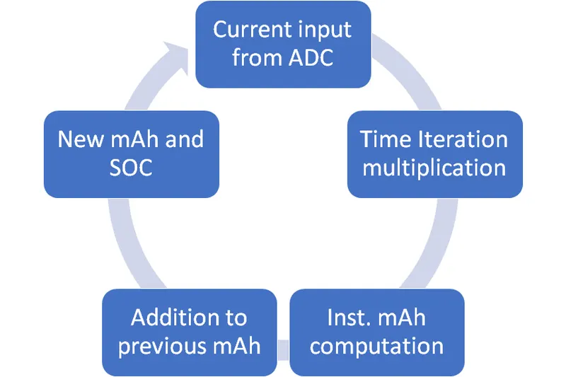
Fig. 2 : Coulomb Counting Algorithm

Hence, the SOC and capacity (mAh) results will be plotted and compared.

Limitations of Coulomb Algorithm : The current can be measured majorily in two ways for the use in algorithm either by shunt resistor or by hall effect sensor. Hall effect sensor is not very accurate since it works on change in magnetic flux and in dc current change in magnetic flux is very low. In case of shunt resistor, heat dissipation takes place, since it is in series. Now, this heat dissipation alters the value of resistance and causes deviation of readings from true measurement. These deviations pile up as additive element in the Battery management system (BMS) algorithm. Also, deviations due to Analog to Digital Converter (ADC) also causes issues in obtaining actual reading. Thus, coulomb counting algorithm has limitations in terms of accuracy. The golden value for SOC estimation is SOC by OCV lookup table but it only works correctly in idle condition when cell polarization is zero. Thus, we need some other suitable algorithm for dynamic SOC calculation. Let's now look at extended kalman filter algorithm.

Kalman Filter Algorithm : This is the most commonly used algorithm in small budget friendly electric vehicles. This type of algorithm uses mathematical stochastic approach to correct the value of output. This algorithm found it's early applications in space science. In rockets, there is need to continuously monitor temperature of engine, but due to high temperature sensor couldn't be placed inside it. Thus, a sensor near to the desired place was kept and temperature of the engine was predicted through extended kalman filter. The other way, in which it can be used is to predict the accurate value based on inputs from multiple sensors. We will use this approach. In this approach, a new state (x(k)) is calculated through previous state (x(k-1)) through one of the sensor. Now, since this sensor has measurement noise, we will use data from other sensor to correctly predict the value. For that, we calulate the value of other sensor from the input reading of this sensor. The other sensor variable is also known as the state observer. This computed value is compared with actual value of the other sensor. Based on the difference between them, value is corrected. In layman's language, this algorithm takes mean of values from different sensors to correctly predict the output. Following, is the general block diagram of the algorithm -

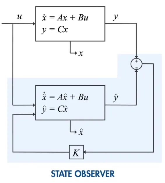
Fig. 3 : Kalman Filter Block Diagram

In, our case we will use coulomb counting to predict value of new capacity(Ah) and correct it by voltage measurement. Referring to the diagram, in our case x is capacity used (Ah), which is calculated from current input from ADC by multiplying it with time iteration. This, instantaneous Ah is added to previous state (x(k-1)) to get new capacity used (x(k)). Now, this new Ah is used to calculate voltage from the SOC-OCV regression fit by including voltage drop due to polarization. The value of voltage from this is used to compare the value from the actual voltage reading. Based on the difference in actual and computed voltage, state value(x(k)) is corrected and kalman gain (K) is adjusted. This state value is used to calculate the next state value. This is how the algorithm works. It is better since here input from two sensors is taken where as in coulomb counting, input from only one sensor is taken.

Limitations of Kalman Filter Algorithm : The kalman filter algorithm can only be used for linear systems due to gaussian distribution function assumption. And battery system in electric vehicle powertrain is highly non-linear. The solution to this is -

Extended kalman Filter Algorithm : In order to use kalman filter algorithm for non-linear systems, kalman filter is applied locally by using jacobian matrix. There are other methods too such as unscented kalman filter, particle filter but they are complex and have high computation cost. For, the sake of simplicity and application in low speed electric vehicles we will use extended kalman filter algorithm.

MATLAB Code :

clear all
close all
clc

% Loading the data
soc_data = load('SOC by OCV Test.txt');
method = soc_data(:,2);
mV = soc_data(:,3);
Inst_mAh = soc_data(:,5);
mAh(1) = Inst_mAh(1);

% mAh computauion for SOC-OCV Relationship
j = 1;

for i = 1:length(Inst_mAh)
   if(method(i)==3 && i>1 && mV(i)>=2800)
       j = j + 1;
       mAh(j) = mAh(j-1)+Inst_mAh(i);
       V(j) = mV(i)/1000;
   end
end

Total_mAh = -mAh(j);

for i = 1:length(mAh)
    Remaining_mAh(i) = Total_mAh + mAh(i);
    soc(i) = (Remaining_mAh(i)/Total_mAh)*100;
end

%plotting capacity vs voltage
figure(1)
mAh = -mAh;
plot(mAh,V)
xlabel('Used Capacity (Ah)')
ylabel('Open Circuit Voltage (V)')
axis([0 2500 2.8 4.5])

%SOC Prediction function
% Polynomial fit of the SOC data
co_effs_voltage_fit_soc = polyfit(soc,V,4);
predicted_voltage_fit_soc = polyval(co_effs_voltage_fit_soc, soc);

% Least square error of fit
Error_fit_soc = (V - predicted_voltage_fit_soc).^2;
LSE_fit_soc = sum(Error_fit_soc)

%Plot actual and fit comparison
figure(2)
plot(soc,V,soc,predicted_voltage_fit_soc)
set(gca, 'XDir','reverse')
xlabel('State of Charge (%)')
ylabel('Open Circuit Voltage (V)')
legend('actual','predicted')

%soc variable split formations
j = 1;
k = 1;
for i = 1:length(soc)
    if(soc(i)>5)
       soc1(j) = soc(i);
       V1(j) = V(i);
       j = j + 1;
    else 
       soc2(k) = soc(i);
       V2(k) = V(i);
       k = k + 1;
    end
end

% Polynomial fit of the SOC 1 data
co_effs_voltage_fit_soc_1 = polyfit(soc1,V1,4);
predicted_voltage_fit_soc_1 = polyval(co_effs_voltage_fit_soc_1, soc1);

% Least square error of fit
Error_fit_soc_1 = (V1 - predicted_voltage_fit_soc_1).^2;
LSE_fit_soc_1 = sum(Error_fit_soc_1)

% Polynomial fit of the SOC 2 data
co_effs_voltage_fit_soc_2 = polyfit(soc2,V2,4);
predicted_voltage_fit_soc_2 = polyval(co_effs_voltage_fit_soc_2, soc2);

% Least square error of fit
Error_fit_soc_2 = (V2 - predicted_voltage_fit_soc_2).^2;
LSE_fit_soc_2 = sum(Error_fit_soc_2)

new_predicted_V_soc = horzcat(predicted_voltage_fit_soc_1,predicted_voltage_fit_soc_2);

%Plot actual and fit comparison
figure(3)
plot(soc,V,soc,new_predicted_V_soc)
set(gca, 'XDir','reverse')
xlabel('State of Charge (%)')
ylabel('Open Circuit Voltage (V) (Split Prediction)')
legend('actual','predicted')

Total_LSE_soc = LSE_fit_soc_1 + LSE_fit_soc_2

%mAh Prediction function
%mAh variable split formations
l = 1;
m = 1;
for i = 1:length(mAh)
    if(l < j)
       mAh1(l) = mAh(i);
       l = l + 1;
    else
        mAh2(m) = mAh(i);
       m = m + 1;
    end
end

% Polynomial fit of the mAh 1 data
co_effs_voltage_fit_mAh_1 = polyfit(mAh1,V1,4);
predicted_voltage_fit_mAh_1 = polyval(co_effs_voltage_fit_mAh_1, mAh1);

% Least square error of fit
Error_fit_mAh_1 = (V1 - predicted_voltage_fit_mAh_1).^2;
LSE_fit_mAh_1 = sum(Error_fit_mAh_1)

% Polynomial fit of the mAh 2 data
co_effs_voltage_fit_mAh_2 = polyfit(mAh2,V2,4);
predicted_voltage_fit_mAh_2 = polyval(co_effs_voltage_fit_mAh_2, mAh2);

% Least square error of fit
Error_fit_mAh_2 = (V2 - predicted_voltage_fit_mAh_2).^2;
LSE_fit_mAh_2 = sum(Error_fit_mAh_2)

new_predicted_V_mAh = horzcat(predicted_voltage_fit_mAh_1,predicted_voltage_fit_mAh_2);

%Plot actual and fit comparison
figure(4)
plot(mAh,V,mAh,new_predicted_V_mAh)
xlabel('Used Charge(Ah)')
ylabel('Open Circuit Voltage (V)(Split Prediction)')
legend('actual','predicted')

%soc calculation for DST project
% Loading the data
dst_data = load('DST_80_SOC.txt');
type = dst_data(:,7);
V_dst = dst_data(:,10);
I_dst = dst_data(:,9);
time_iteration = dst_data(:,5);

initial_values_dst_cc = [0 0.8*Total_mAh 80];
time_dst_cc(1) = initial_values_dst_cc(1);
mAh_dst_cc(1) = initial_values_dst_cc(2);
soc_dst_cc(1) = initial_values_dst_cc(3); 
k = 1;
j = 1;

%Coulomb counting method
for i = 1:(length(type)-1) %leaving last value due to high garbage value of time iteration
    if(type(i) == 7 && i>1)
     mAh_dst_cc(j+1) = mAh_dst_cc(j) + ((time_iteration(i)*I_dst(i)/3600)*1000);
     soc_dst_cc(j+1) = (mAh_dst_cc(j+1)/Total_mAh)*100;
     time_dst_cc(j+1) = time_dst_cc(j) + time_iteration(i);
     j = j+1;
        if(soc_dst_cc(j)<=10)
            break;
        end
    end 
end

%extended kalman filter method
initial_values_dst_ekf = [0 0.2*Total_mAh 80];
mAh_dst_ekf(1) = initial_values_dst_ekf(2);
soc_dst_ekf(1) = initial_values_dst_ekf(3); 
time_dst_ekf(1) = initial_values_dst_ekf(1);

k = 2;
result = 0.2*Total_mAh;
mAh1_max = mAh1(end);
for i = 1:(length(V_dst)-1) %leaving last value due to high garbage value of time iteration
    if(type(i) == 7 && i>1)    
     f = @(x,u)(x -(((u*time_iteration(i))/3600)*1000)); %using coulumb counting according to iteration time
     if(result<=mAh1_max)
        h = @(x,u)(co_effs_voltage_fit_mAh_1(1)*(x^4) + co_effs_voltage_fit_mAh_1(2)*(x^3) + co_effs_voltage_fit_mAh_1(3)*(x^2) + co_effs_voltage_fit_mAh_1(4)*(x^1) + co_effs_voltage_fit_mAh_1(5) + ((u+0.1)*(18/1000)));
     else   
        h = @(x,u)(co_effs_voltage_fit_mAh_2(1)*(x^4) + co_effs_voltage_fit_mAh_2(2)*(x^3) + co_effs_voltage_fit_mAh_2(3)*(x^2) + co_effs_voltage_fit_mAh_2(4)*(x^1) + co_effs_voltage_fit_mAh_2(5) + ((u+0.1)*(18/1000)));    
     end
     V_test(k) = V_dst(i);
     obj = extendedKalmanFilter(f,h,result);
     correct(obj,V_dst(i),I_dst(i))
     result = predict(obj,I_dst(i));
     mAh_dst_ekf(k) = result;
     soc_dst_ekf(k) = (1-(result/Total_mAh))*100;
     time_dst_ekf(k) = time_dst_ekf(k-1) + time_iteration(i);
     if(soc_dst_ekf(k)<=10)
         break;
     end
     k = k+1;
    end
end

figure(5)
plot(time_dst_cc,soc_dst_cc,time_dst_ekf,soc_dst_ekf)
legend('Coulomb Counting','Extended Kalman Filter')
xlabel('Time Stamp Iteration of DST Test')
ylabel('State of Charge(%)')

%Difference in SOC values
for i=1:length(time_dst_ekf)
   difference_soc(i) = soc_dst_cc(i)-soc_dst_ekf(i);
end    

figure(6)
plot(time_dst_ekf,difference_soc)
xlabel('Time Stamp Iteration of DST Test')
ylabel('SOC(Coulomb counting) - SOC(Extended Kalman Filter)')

figure(7)
plot(time_dst_cc,mAh_dst_cc,time_dst_ekf,Total_mAh - mAh_dst_ekf)
legend('Coulomb Counting','Extended Kalman Filter')
xlabel('Time Stamp Iteration of DST Test')
ylabel('Capacity Used(mAh)')

%Difference in mAh values
for i=1:length(time_dst_ekf)
   difference_mAh(i) = mAh_dst_cc(i)-(Total_mAh - mAh_dst_ekf(i));
end    

figure(8)
plot(time_dst_ekf,difference_mAh)
xlabel('Time Stamp Iteration of DST Test')
ylabel('mAh(Coulomb counting) - mAh(Extended Kalman Filter)')

Discussion of Code : Initially, we clear all variables, workspace and close all the windows. Then, we loaded the low current data in the matlab workspace to create SOC-OCV profile and allot suitable names to parameters being withdrawn. We will be using voltage values, current values, time iteration to compute Ah and in turn State of Charge. There are different cycles which have been written in excel file of the experiment. We will only use the one where it is being continuously discharged at 0.05A. Then, we will use for loop to estimate total mAh consumed till now at each moment, so as to plot the curve and compute the total mAh of the cell. After computing total Ah, we will divide total mAh at every iteration with this value and multiply by 100 to get SOC in percent at each instant. Then, we will plot capacity used vs voltage of the cell to verify discharge characteristics. We achieved following discharge characteristics which is similar to general lithium-ion cell characteristics.

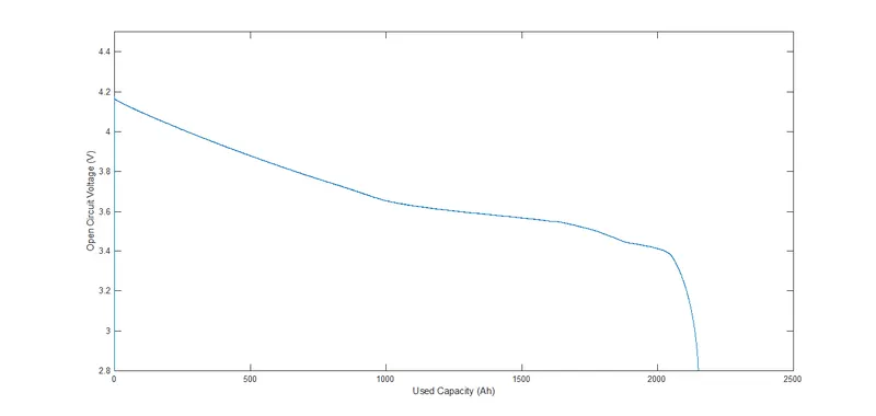
Fig. 4 : OCV vs Ah at 0.05C Rate

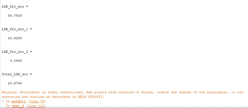
Now, since we have the soc vs ocv relation, we can use regression fit to create a polynomial corresponding to discharge curve of the cell. For, this pupose we will use polyfit and polyval function. We will use polynomial of degree 4 since that is most commonly used for lithium cell discharge characteristics. Then, least square errors is also computed and plot of actual vs regression fit function is plotted. As we can see that least square error, is 83.75 and there is deviation between actual and predicted value towards the end as shown in the figure below -

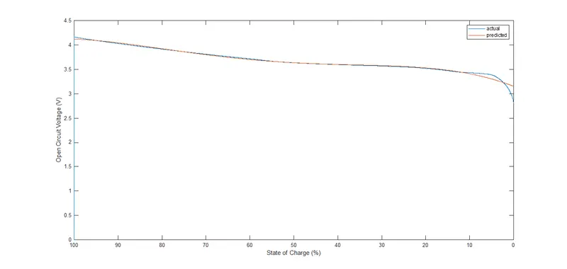
Fig. 5 : OCV vs SOC regression fit comparison

To correct this deviation towards the end which is due to sudden drop in voltage towards the end of the SOC of the cell due to sudden increase in polarization (represented by internal resistance), we will split the function in two parts from the point where deviation starts happening. As we can see in the plot, it starts happening from almost SOC = 5, we will split the curve into two curves through for loop. After that we will separately do regression fit for both the curves and use horzcat command to combine polynomial output of both curves to compare it with the actual curve. Also, we will add least square error of both the curves to calculate the total least square error. This time total least square is 20.6764 which is almost 75% reduction in error. We can see this in the plot where actual and predicted values are almost equal as shown in the figure below-

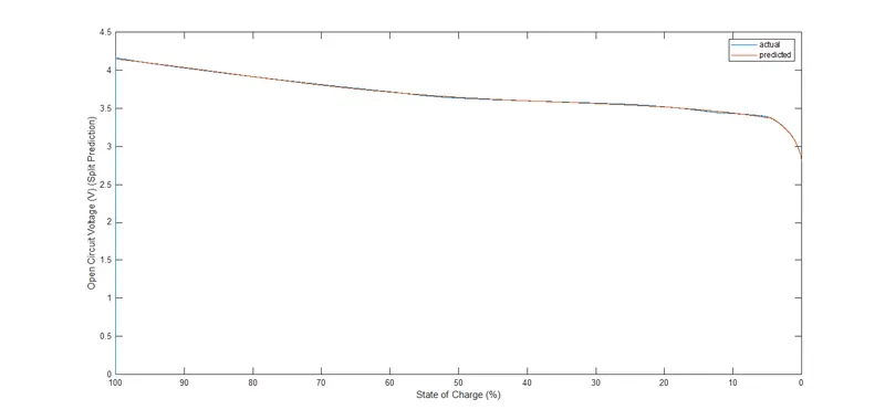
Fig. 6 : OCV vs SOC regression fit split comparison

Now, we will implement coulomb counting and extended kalman filter algorithm for DST cycle data. Firstly, we will load dst cycle data and assign suitable variable names to data similar to what we did in plotting SOC-OCV curve. Now, this data is for DST cycle test with cell of 80% SOC at the start. Hence, we will assign initial conditions to the result matrices according to the given condition. Then, we will use for loop to compute SOC through coulomb counting algorithm. At each iteration step we will multiply current value with the corresponding time iteration and convert the units into mAh to get instantaneous mAh value. Then, we will add this to previous mAh value to compute total capacity used. Since, current is negative for discharge, we will get reduced mAh at almost each step (except for regenerative braking in DST cycle). This value of reduced mAh at each step will be used to compute SOC by dividing it by total SOC. The loop breaks when SOC reduces below 10, since cell is never recommended below certain voltage or SOC (internationally generally it is 2.8V and in India generally it is 3.0V). Thus, we values of SOC for the DST cycle discharge.

Now, we will implement extended kalman filter algorithm and then compare the results for both the algorithms. Here, approach is different. As per discussed in project outline, x is the mAh consumed till the iteration, u is the current input from ADC and y (or measurement signal output) is voltage. Here, also we will first initialize the states with the given parameter of 80% SOC (translates to 20% of used charge). Then, we will use for loop. At each iteration of loop, first it encounters state transition function where from previous state, new state is calculated. Previous state is total mAh used till the last stage and new mAh is addition of product of instantaneous current with time to the last state (as in the case of coulomb counting). Now, for measurement function there will be an if-else case, since we had split the SOC-OCV regression fit function into two parts. If, the used mAh is less than second split function, we will use first split function otherwise we will use the second split function. Then, we will correct the value of the calculated result by putting in the measured value. The result after correction will be used to calculate SOC by dividing it by total_ah and subtracting it by 1. In both the algorithms we are storing time instant values too for the sake of plotting the graphs. At the end we will plot the graphs to compare both algorithms. First, we compared SOC and mAh through both the algorithms and then their corresponding differences.

Algorithms Comparison :

1. First, we will compare SOC results from both the algorithms as shown below. As we can see that almost they are showing same results except for minor deviations. But, we will get clear picture on difference plotting.

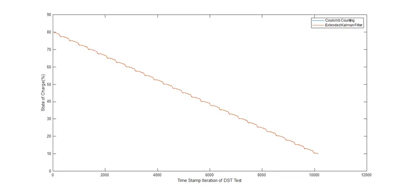
Fig. 7 : SOC vs Time Iteration Comparison of DST Cycle

on zooming, we get to know some minor differences

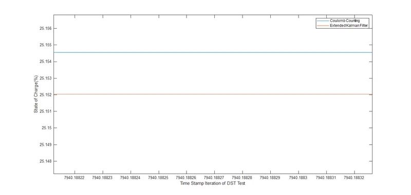
Fig. 8 : SOC vs Time Iteration Comparison of DST Cycle (Zoom View)

2. Next, we will compare capacity used results from both the algorithms as shown below. As we can see that almost they are showing same results except for minor deviations. But, we will get clear picture on difference plotting. Here, difference in value will be more since SOC was %age based but it is absolute value based.

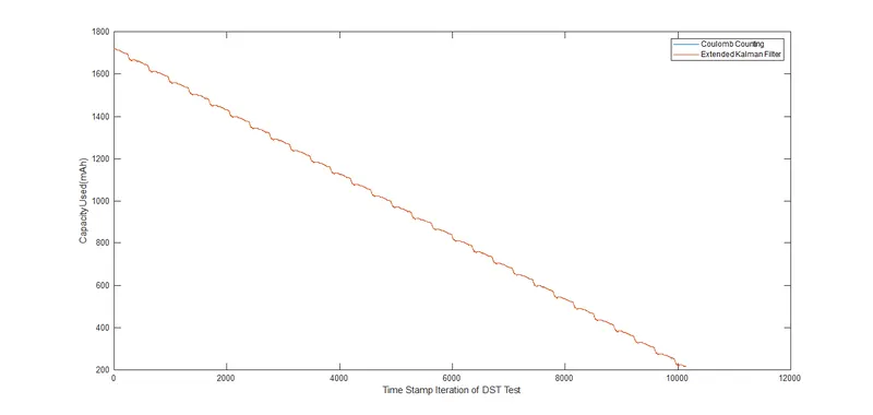
Fig. 9 : Capacity used (mAh) vs Time Iteration Comparison of DST Cycle

On zooming, we get to know more clarity on the differences as below -

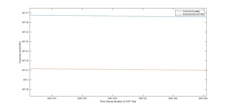
Fig. 10 : Capacity used (mAh) vs Time Iteration Comparison of DST Cycle (Zoom View)

3. Now, we will see plot of difference between SOC of both the algorithms. As we can see in the plot, that in case of coulomb counting there is continuous increase in difference due to continual measurement noise addition, and which reinforces the theorotical importance of kalman filters in reducing the noise addition errors in results by continually adjusting values from output of the other sensors.

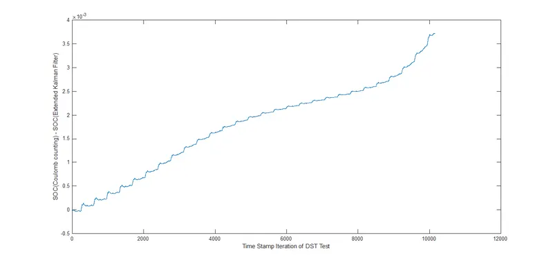
Fig. 11 : SOC Difference Comparison of Algorithms

4. We can also plot this comparison for capacity used and it will give similar curve since SOC is an indirect expression of capacity used.

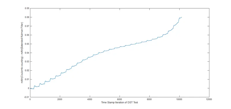
Fig. 12 : Capacity Used (mAh) Difference Comparison of Algorithms

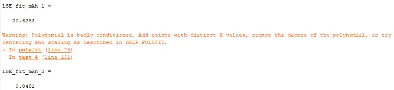
Command Window :

Conclusion and Future Scope : Thus, as shown above extended kalman filter can be an effective algorithm to weed out additive measurement noises and process noises which otherwise appear in the case of coulomb counting algorithm. This is due to the fact, since it is adjusting value based on measurement from some other signal (in this case voltage). So, results in case of extended kalman which takes input from 2 signals is more accurate than results derived from one signal input. Also, this is the reason for it's popularity since it's cost-effective and accurate and thus meets the engineering goals. Though, with huge data neural network based algorithm is more accurate but it's implementation is very costly (atleast locally). Also, we need huge data to make neural networks a success, which again reflects the chiken-egg problem. So, in order for smooth transition to electric vehicles, we need to start from kalman filters and gradually to artificial intelligence based. There are also, some scope of improvements in this algorithm. Firstly, extended kalman filter is accurate when function varies linearly locally. But, if there are big non-linearities it won't perform as good. For, that we have algorithms like unscented kalman filter and particle filter but they are bit complicated and expensive to implement on microprocessors whereas this type of algorithm can be fairly easily deployed on a microprocessor. Secondly, internal resistance is assumed constant, which is not the case always. Hence, correction of internal resistance from a lookup table is desired. In this case, didn't have internal resistance lookup table for DST discharge and it needs sophisticated lab equipments to measure it. Thirdly, all the SOC-OCV curves are calculated with very low currents but still have some polarization in them. The exact OCV is voltage after cell has rested for about 20 minutes. Thus, these are my conclusions and future scope on the project. I have been active in the field of electric vehicles for around 7 years, connect with me at [email protected]

Thanks!!

References :

1.Dişçi, F.N., El-Kahlout, Y. and Balıkçı, A., 2017, November. Li-ion battery modeling and SOC estimation using extended Kalman filter. In 2017 10th International Conference on Electrical and Electronics Engineering (ELECO) (pp. 166-169). IEEE.

2.Zhi, L., Peng, Z., Zhifu, W., Qiang, S. and Yinan, R., 2017. State of charge estimation for Li-ion battery based on extended Kalman filter. Energy Procedia, 105, pp.3515-3520.

3.How, D.N., Hannan, M.A., Lipu, M.H. and Ker, P.J., 2019. State of charge estimation for lithium-ion batteries using model-based and data-driven methods: A review. IEEE Access, 7, pp.136116-136136.

4.Saqli, K., Bouchareb, H., Oudghiri, M. and M'sirdi, N., 2019, September. An overview of State of Charge (SOC) and State of Health (SOH) estimation methods of Li-ion batteries. In IMAACA 2019.

5.Xiong, R., Cao, J., Yu, Q., He, H. and Sun, F., 2017. Critical review on the battery state of charge estimation methods for electric vehicles. Ieee Access, 6, pp.1832-1843.

6.Yao, Q., Lu, D.D.C. and Lei, G., 2018, November. A Simple Internal Resistance Estimation Method Based on Open Circuit Voltage Test Under Different Temperature Conditions. In 2018 IEEE International Power Electronics and Application Conference and Exposition (PEAC) (pp. 1-4). IEEE.

7.Tesla Battery Day – 2020 : https://youtu.be/l6T9xIeZTds