Exhaust Port Challenge

Conjugate Heat Transfer:

The physical phenomenon where heat transfer takes place simultaneously in both solids and fluids is termed as conjugate heat transfer. However, the modes of heat transfer in solids and fluids vary. In solids, the heat transfer is predominantly by conduction mode and while in fluids it is governed by convection.

Conduction in solids is governed by Newton’s Law of heat conduction and depends highly upon the heat conductivity of solid and temperature gradient.

` q = k grad T `

Where `q` = heat flux

`k` = thermal conductivity

`grad T` = temperature gradient

While convection in fluids is governed by Newton’s Law of cooling and is proportional to temperature difference.

`q = h(T_s – T_f)`

Where `q` = heat flux or heat transfer rate

`h` = convection heat transfer coefficient

`T_s` = Temperature of surface

`T_f` = Temperature of fluid surrounding the solid medium

When a fluid flows over a surface of solid the fluid layer next to the surface boundary (layer In contact with surface) comes to a stationary halt and velocity of such fluid layer is zero, this condition is known as no-slip condition. And because of friction the velocity of successive adjacent layers is always greater than that of the layers below. As a result a velocity profile is formed.

A similar phenomenon occurs for temperature also. When bodies of different temperatures are brought in contact with each other, heat transfer will take place till both bodies are in equilibrium (attain same temperature). Therefore, a fluid and surface will have same temperature at the point of contact. This is known as no- temperature-jump condition. Also, due to presence of temperature difference in adjacent layers, a profile similar to velocity profile is formed, which is termed as temperature profile.

To deal this combined phenomenon two dimensionless numbers are often used Nusselt’s Number and Prandlt’s Number.

· Nusselt’s Number:

It is ratio of heat fluxes of convection and conduction.

`Nu = frac{q_(conv)}{q_(cond)} = frac{h grad T}{k grad T/L} = frac{hL}{k}`

Physically, it signifies the amount of heat convection taking place in fluid layer with respect to conduction. The more the value of `Nu` suggests the better convection.

· Prandlt’s Number:

It is defined as the ratio of diffusivity of momentum to diffusivity of heat.

`Pr = frac{mu C_p}{k}`

For a fluid with `Pr` greater than 1 would mean that the momentum layer is dominant than thermal layer and value of `Pr` less than 1 would mean vice versa.

Control of these heat fluxes are required to design effective heat exchangers, heaters or coolers. Some applications of CHT are heat exchangers (shell and tube), evaporators, and heat sinks. The fluid in these processes helps in carrying energy (temperature) to large distances. And solids acts as boundary to keep the fluids separate.

To further study the effect of CHT flow of hot gases through exhaust port is taken up.

Solving & modelling approach:

• Geometry:

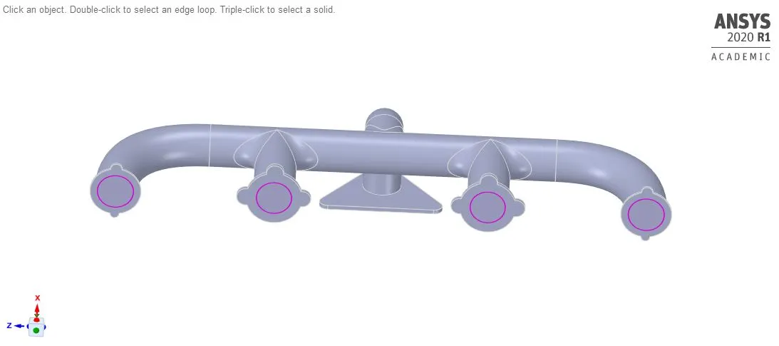
1. For correctly meshing the geometry, the volume pertaining to fluid flow was marked as a separate component. The same action was performed for solid volume. Finally, these two volume components are moved to a new volume body.
2. Share Topology Function: It was ensured that both solid-volume and fluid-volume share topology so that a conformal mesh is generated during mesh. A red circle around the interface of solid-fluid volume ensures that the topology is being shared.

• Meshing:

1. Named Selection: Before generating mesh named selection was created on components of geometry.
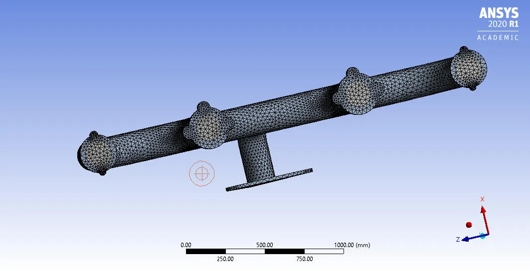
2. Base Mesh: In this scenario no refinement was added and system generated default mesh settings were used to obtain the solution.
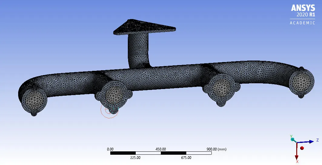
3. Refined Mesh: Two types of refinement were done to obtain a finer mesh.
   • Body Sizing: A sizing method was added to the solid volume and element size of 16mm was chosen.
     • Capture Curvature was set to Yes to resolve the curvature around the circular section of pipe.
   • Inflation layer: A global inflation layer was added so that the physics near the solid fluid interface can be captured.
   • Specification of inflation layer
     • First layer thickness of 0.08 mm was chosen
     • Growth rate of 1.2 with 5 maximum layers.

Base Mesh

Refined Mesh

• Solver and Solution configuration: For both base mesh and refined mesh following solver settings were used:

1. Inlet Velocity = 5 m/s
2. Inlet Temperature = 700K
3. Heat Transfer Coefficient of solid surface = `20 W / m^2 K`
4. Solver = Pressure based steady state
5. Turbulence model = k-omega SST.
6. First Layer thickness for Refined Mesh = 0.08mm

Results:

Wall Y+ values of base line mesh

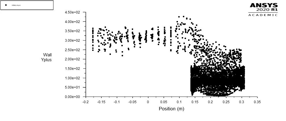
Wall Y+ values of refined mesh

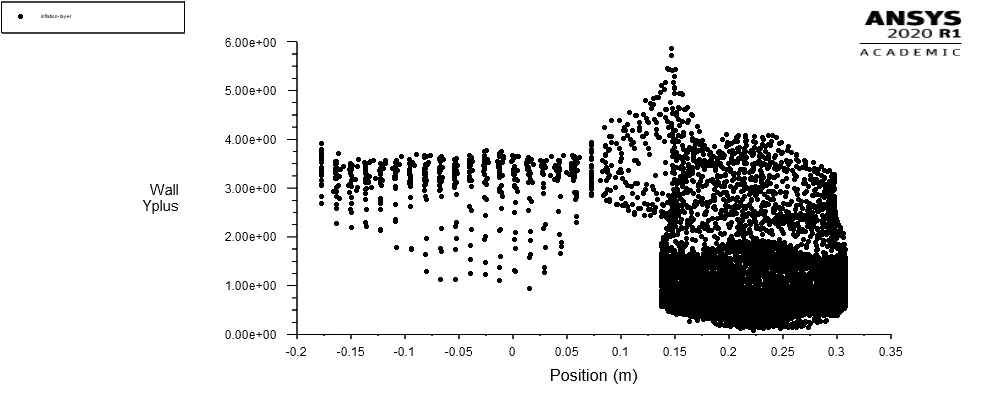
A quick comparison between the Y+ values of base mesh and refined mesh indicates that capturing physics near the boundary wall is essential. For capturing the same, giving special attention to below two processes becomes prudent.

1. Mesh Resolution
2. Turbulence Model Selection

Mesh Resolution:

Mesh Resolution plays a crucial role in any CFD solution pipeline. It not only helps in model selection but also reduces residual errors in the solution. Moreover, achieving a grid-dependent solution is also an integral step which starts with a finely resolved mesh. Considering a target y+ of 1mm calculation of first layer thickness was done in this study.

Turbulence Model Selection:

Out of several other turbulence models available in ANSYS, the two most popular models are k-epsilon and k-omega.

The k-epsilon model creates a wall function or bridge between the near-wall layers of the solid and the layers far from the wall surface. As a result, the resolution of flow in the buffer and sub-viscous layers does not take place, and hence the wall function takes precedence in deriving the solution. The advantage of such a method applies to cases where viscous and sub-layer effects are not of importance.

Whereas, the k-omega SST model even though being a low Reynold’s number model, can integrate the solution in the laminar sub-layer. As a result, fluid flows in which processes like heat exchange and adverse pressure gradients are involved such models are favourable. The valid range of Y+ value for near wall treatment is 1 to 5.

Considering the above two factors, simulation for the current study, using a k-omega SST model to a finely resolved mesh with a first-layer thickness of 0.08 mm was performed.

The obtained Y+ values confirm the results obtained from the baseline mesh are crude in form. For most of the points in the fluid flow, the Y+ values lie in the range 5 to 30 in this case. As mentioned earlier, this range is not valid for the k-omega model or models where near wall treatment of flow is of importance. Whereas, in the case of refined mesh, the Y+ values lie in between 0 to 5. Hence, the results from the baseline mesh are unacceptable as it follows neither of the log-law nor defect-law.

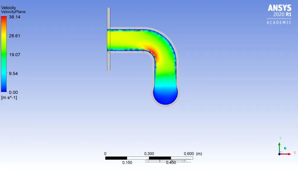
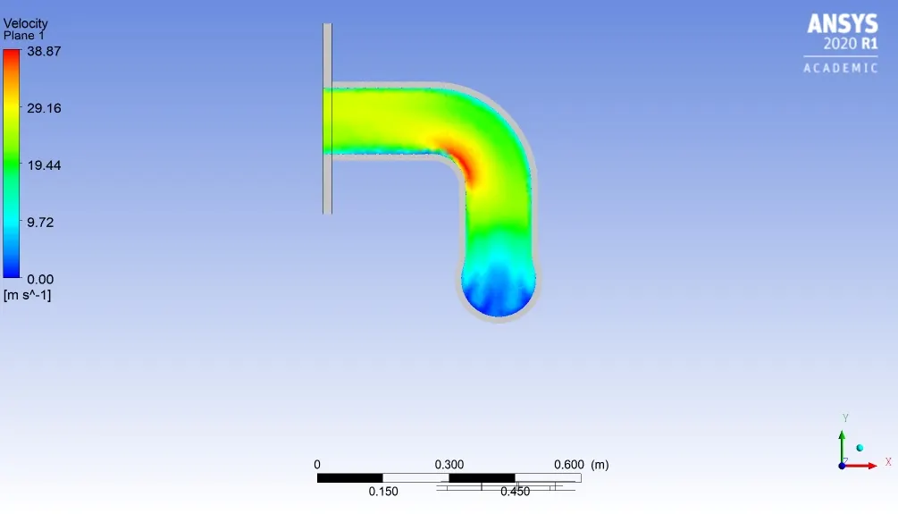
Velocity Contour of Base line Mesh and Refined mesh

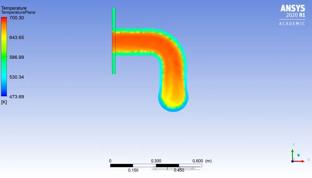
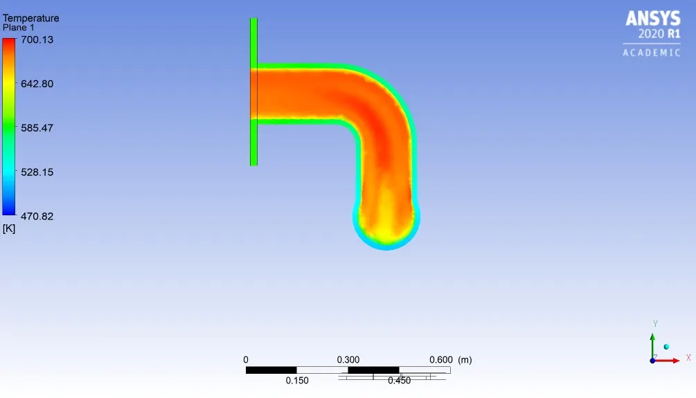
Temperature Contour of Base line Mesh and Refined mesh

Wall Heat Transfer Coefficient Contour of Base line Mesh and Refined mesh

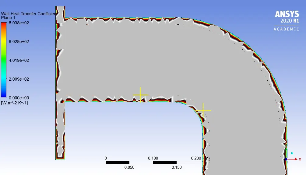
Probe Point before bend showing wall heat transfer coefficient

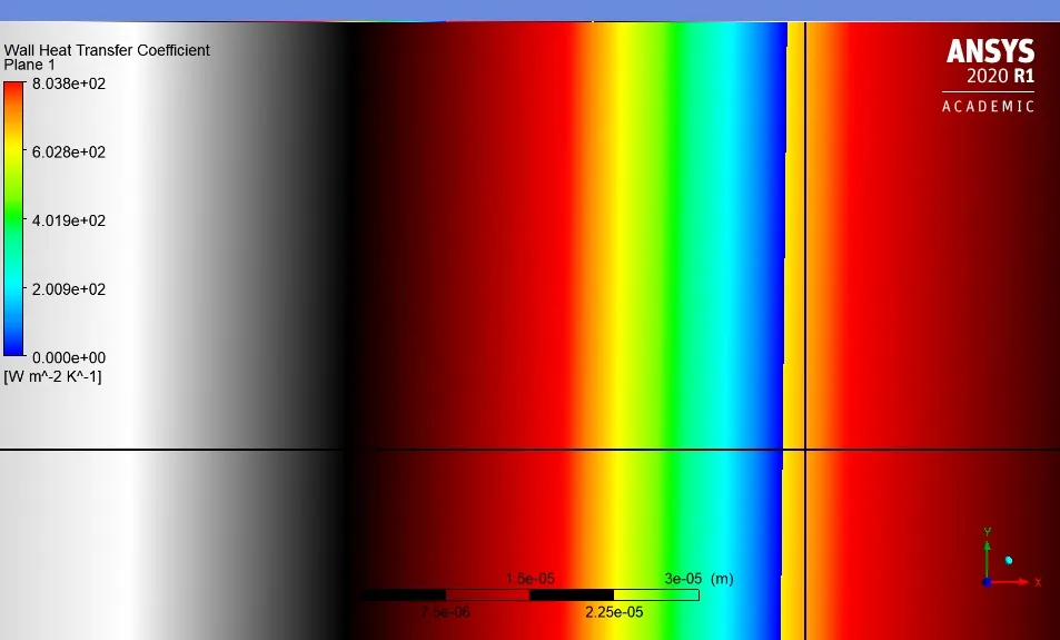
Probe Point at bend showing wall heat transfer coefficient

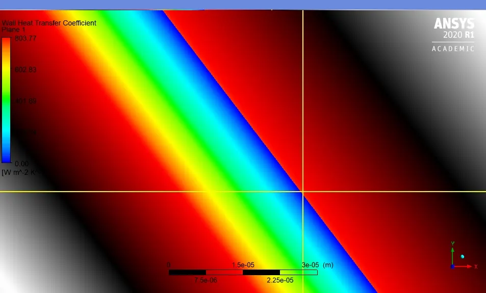
Probe Point after bend showing wall heat transfer coefficient

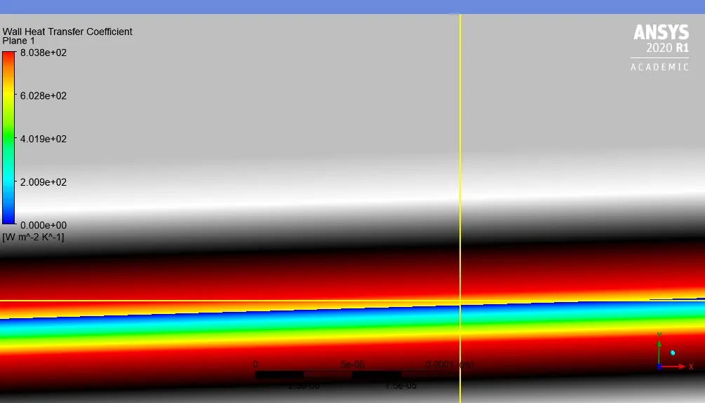
Furthermore, deriving a similar conclusion will not be erroneous if we verify the results from contour plots of velocity, temperature and wall heat transfer coefficient.

• As the dimensions of inlet and outlet do not differ much, the velocity of the fluid at the outlet will be higher to conserve mass. And the same can be observed in the velocity contour plots.
• The predicted velocity at the wall boundary is inaccurate in the case of baseline mesh, even though the velocity at the outlet prediction is almost similar to refined mesh. Due to the absence of a refined mesh in the baseline case, the velocity prediction is inaccurate.
• Furthermore, as observed, the fluid flow starts attaining the maximum velocity as it approaches the bend near the outlet ^[1]. As a result, the fluid flow has a high Reynolds number in this region.
• Placing probe points before, at and after the bend reveals that the value of the wall heat transfer coefficient has increased gradually and it attains maximum value at the elbow. The value decreases as the fluid advances towards the outlet with reduced velocity after the bend. Pressure drop also accompanies this velocity increase.

Location	Heat Tranfer Coefficient
Point before Bend	6.242e+2 [W m^-2 K^-1]
Point at Bend	7.811e+2 [W m^-2 K^-1]
Point after Bend	6.089e+2 [W m^-2 K^-1]

• Due to this increased value of heat transfer coefficient, a large amount of heat transfer takes place from fluid to solid body. Hence, the temperature of the solid is maximum, in and around the bend region.

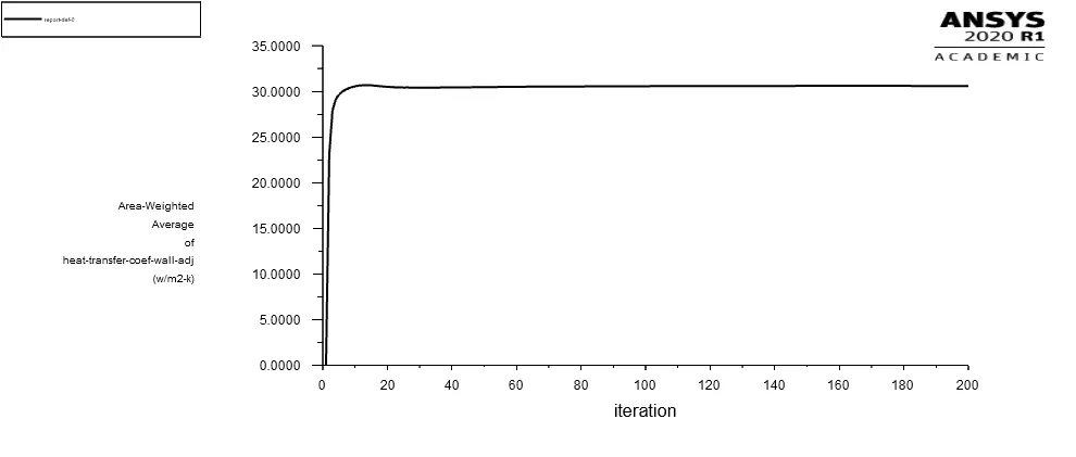
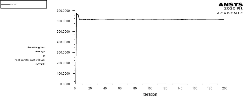
• The area-average wall heat transfer coefficient is less in case of baseline mesh scenario. And as mentioned earlier that the Y+ values for the baseline mesh do not lie in the valid range, helps in ascertaining that the approach in the refined mesh is correct in nature.
• Experimenting for calculating the wall heat transfer coefficient can also help in verifying and validating results from this study.

Overview and Conclusion:

Property	Baseline Mesh	Refined Mesh
Velocity at the outlet	20 m/s	20 m/s
Velocity at bend	38.14 m/s	38.87 m/s
Temperature at the bend	700 K	700 K
Average Wall Heat Transfer Coefficient (in `W/m^2 K`)	30.593377	612.71479
Target Y+	-	1
Number of elements	138378	497569

• Due to the presence of fluid motion heat transfer rate from fluid to the wall surface increases, this is because of convection (forced convection). This fluid motion can be leveraged to either carry heat over large distances or to produce desired heat exchange effect.
• Obtaining more accurate results is possible by further refining the mesh. Since the simulation performed is on an ANSYS Academic Licence, the number of elements cannot exceed beyond 0.5 million. Hence, the refinement of the solution is until these constrained limits only.

References:

[1] Dutta, Prasun & Nandi, Nityananda. (2016). Effect of bend curvature on velocity & pressure distribution from straight to a 90° pipe bend-A Numerical Study. REST Journal on Emerging trends in Modelling and Manufacturing. 2. 103-108.

Link to Ansys files - https://drive.google.com/file/d/1xx3Y1TD6767S_kqmgDR4xxKuH2WIpqOj/view?usp=sharing