Challenge

Exhaust Port Challenge

SSharique Iqbal5 Sept 2020

Aim – Three dimensional CFD analysis of flow through an engine exhaust port.

Introduction –

Understanding of the gas exchange process in an internal combustion engine (ICE) is essential in order to construct efficient engines. In a Diesel engine, of the total available energy, approximately 30-40% of the energy is lost after combustion through the exhaust gases [1].The exhaust part of the gas exchange process involves a highly three-dimensional (3D), turbulent, transonic flow in a complex geometry. When the exhaust valves open, the pressure difference between cylinder and exhaust port is of the order of 500 kPa and the temperature differs with more than 300 K.

The purpose of this study is to perform a Conjugate Heat Transfer (CHT) analysis of a simple engine exhaust port to get a basic understanding of the heat transfer and flow characteristics in an exhaust. The term conjugate heat transfer (CHT) is used to describe processes which involve variations of temperature within solids and fluids, due to thermal interaction between the solids and fluids. The exchange of thermal energy between the two physical bodies is called study of Heat Transfer, the rate of transferred heat is directly proportional to the temperature difference between the bodies. A typical example is the heating or cooling of a solid object by the flow of air in which it is immersed and some other example includes conduction through solids, free and forced convection in the gases/fluids and thermal radiation.

Conjugate heat transfer corresponds with the combination of heat transfer in solids and heat transfer in fluids. In solids, conduction often dominates whereas in fluids, convection usually dominates. Efficiently combining heat transfer in fluids and solids is the key to designing effective coolers, heaters, or heat exchangers. Forced convection is the most common way to achieve high heat transfer rate. In some applications, the performances are further improved by combining convection with phase change (for example liquid water to vapor phase change). For many simulations of real world engineering applications, the predictions of heat transfer properties are as important, if not more important, than the actual flow field. Such scenarios include simulations of heat exchangers, HVAC (Heating, Ventilation and Air Conditioning), combustion/burners, electronics cooling, and many more. In these applications, we are often interested in how heat moves through both the fluid and solid domains, and importantly the transfer of heat across the interface between adjacent domains.

Modelling and Solving approach –

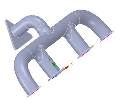
Solid Model – A 3D CAD model was imported in Ansys Spaceclaim.

The volume extraction feature of Spaceclaim was utilized to extract the fluid volume and the topology was shared using the Share feature of Spaceclaim to get conformal mesh between the solid and fluid regions. The geometry was then exported to Ansys Mesher. The model in Spaceclaim is shown below.

Meshing – Two different meshing strategies were utilized. For the baseline mesh no tweaks were made in the Ansys mesher and an automatic mesh generated was utilized in Fluent. When refining, sizing and inflation layers were used for the outer and the inner wall respectively.

The mesh statistics for all the cases are given in the below table.

	Element size (mm) [element type]	Inflation layers used	Number of elements
Case 1	150 [Tetrahedral]	No	137257
Case 2	100 [Hexahedral]	Yes	246455
Case 3	50 [Hexahedral]	Yes	259836

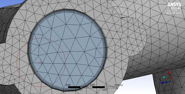
The mesh near the inner wall must be fine enough to capture the boundary layer and heat transfer effects efficiently. This is achieved using appropriate inflation layers. Thus the first cell height of 5 mm has been used for all the computations.

The images of the mesh domain for all the cases are given below –

Case 1

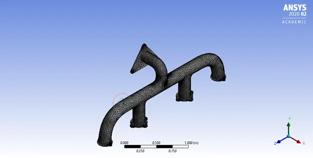
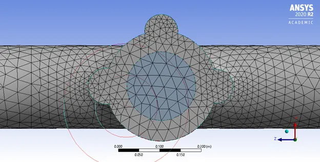
Case 2

Case 3

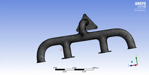
Solver Settings – Ansys Fluent was used as the solver and steady state simulations have been performed using a density based solver. Air was used as the fluid. The inlet velocity was 5 m/s at 800 K.

Boundary conditions – Reynolds number was varied by changing the inlet velocities. The below table highlights the different velocities used.

Name	Boundary conditions
Inlet	Velocity inlet (25 m/s), T = 800 k
Outlet	Pressure outlet (0 Pa)
Outer wall	Convection , h = 20 W/m2K
Inner wall	Coupled
All other walls	Adiabatic

Reynolds Number –

Approximate diameter of the inlet is 82 mm. For calculations, a diameter of 80 mm has been considered.

`Re= (ρVD)/μ=(1.225*5*0.08)/(1.7894e-05)≈28000`

Clearly the flow is turbulent as evident by Reynolds number.

Computational model – As per literature and Ansys Fluent documentation, Realizable k-epsilon model has been used for all the computations.

Spatial Discretization Method – SIMPLE Pressure velocity coupling scheme was used to solve the Navier Stokes Equations. The methods used for spatial discretization of each of the terms is given in the below table –

Term/Equation	Method
Gradient	Least Squares Cell based
Pressure	Second Order
Momentum	Second Order Upwind

Results and Discussion –

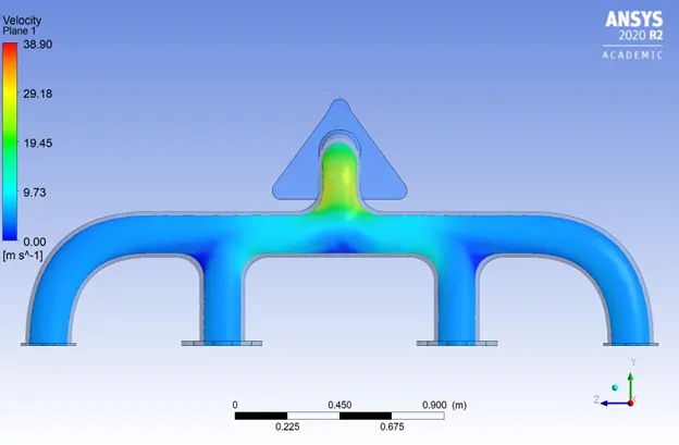
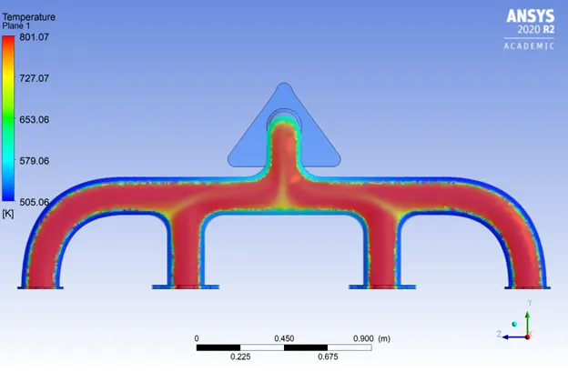
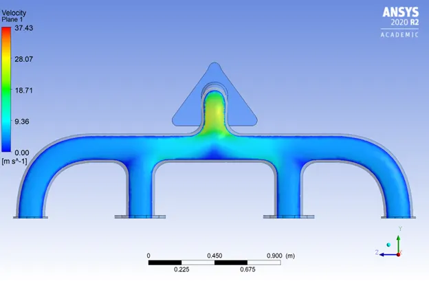
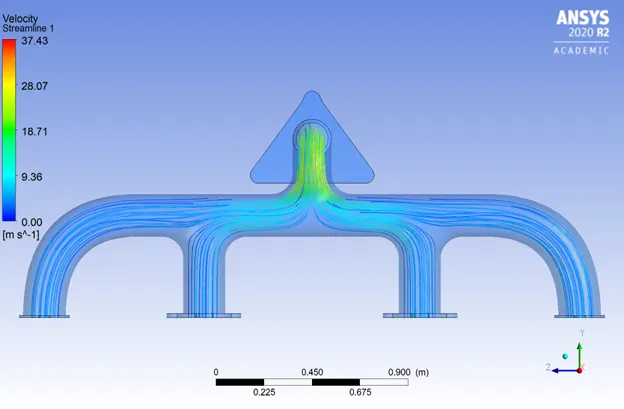
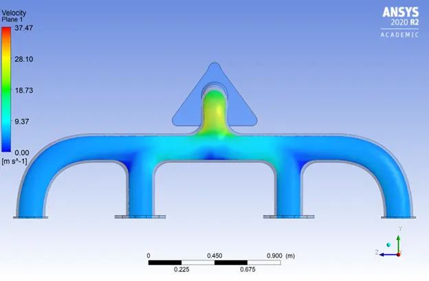
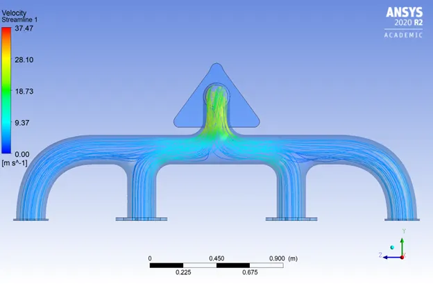
The velocity of the flow is observed to increase near the outlet elbow. This is in agreement with mass conservation. The same is highlighted in the streamline and velocity contour plots.

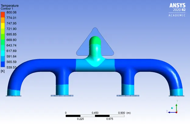
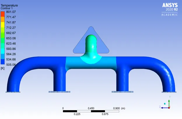
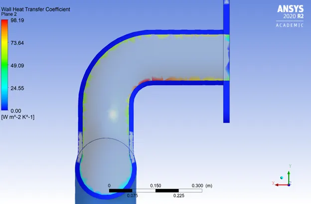
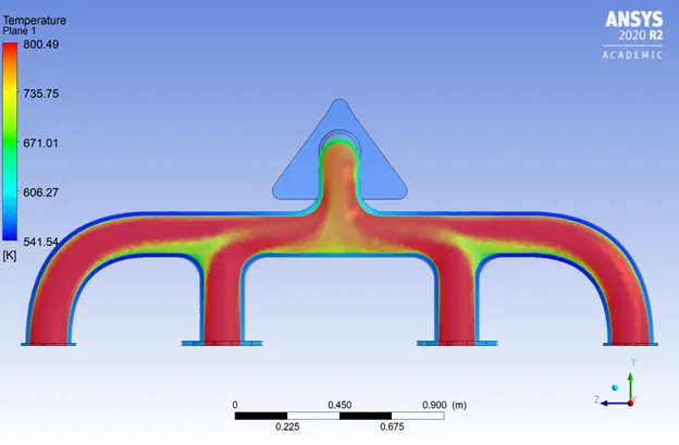
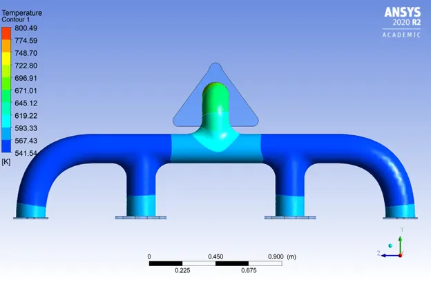
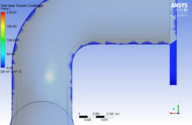
Also, since the heat transfer coefficient is a function of Reynolds number, near the outer elbow the temperature of the outer wall of the pipe shows rapid decrease. The exhaust also loses heat s it reaches the outer elbow.

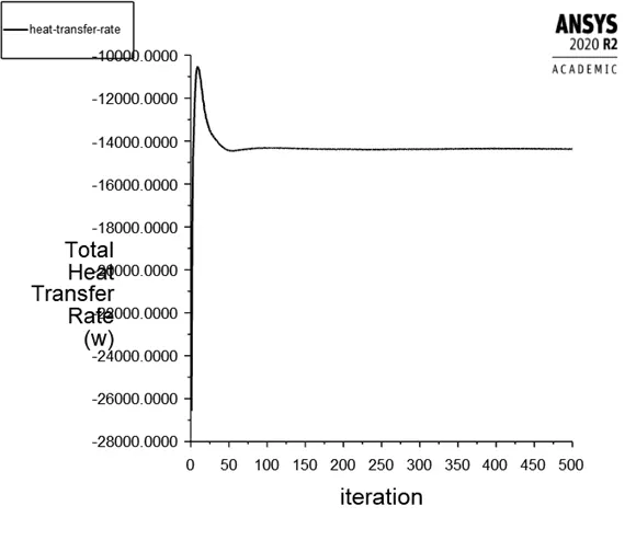
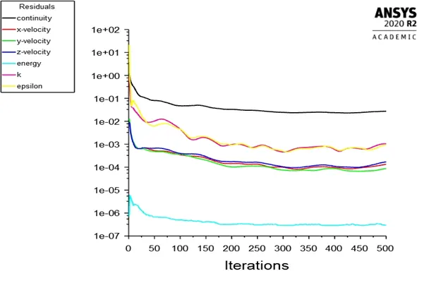
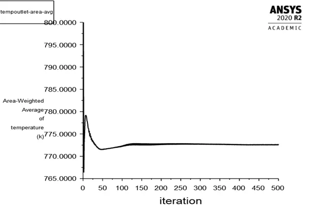
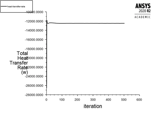
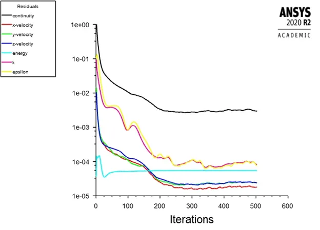
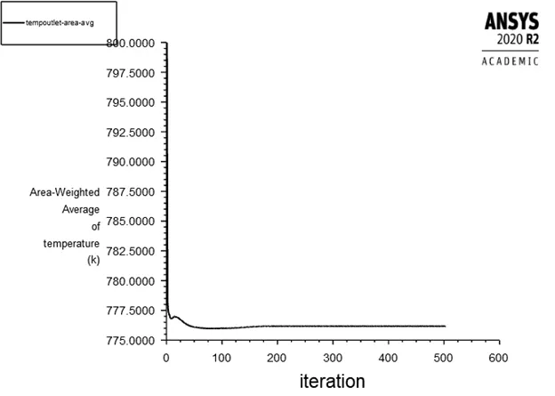
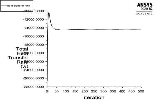
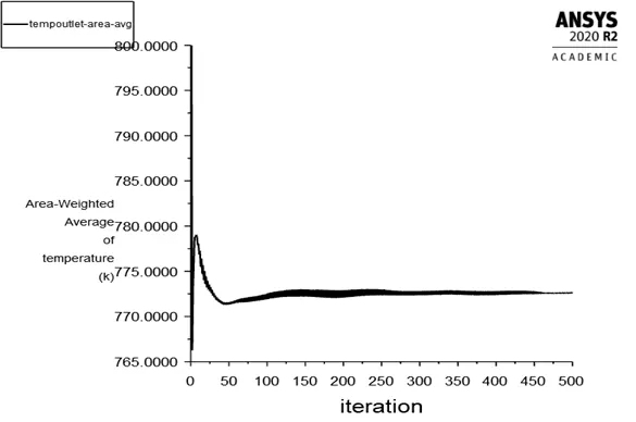
From the heat transfer and the average outlet temperature plots, it can be observed that the solution is converged after about 200 iterations. The entire calculations were, however, performed for 500 iterations.

The mesh independence test was also performed. And it is evident from the comparison of heat lost and average outlet temperature that the results are accurate. The same have been shown in the below table. The negative sign of the heat transfer indicates that heat is lost from the system. All the relevant plots are given below.

	Heat Transfer Rate (W)	Average Temperature at the Outlet face (K)
Case 1	-12498.65	776
Case 2	-14490.82	772.56
Case 3	-14379.73	772.71

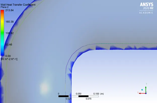
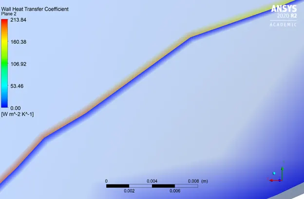
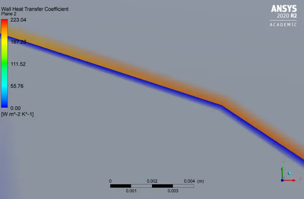
The heat transfer coefficient contour clearly shows high heat transfer coefficient at the inner bend near the outlet elbow. This is because velocity is high in that region, thereby increasing the local heat transfer coefficient.

Verification of heat transfer coefficient – It is equal to:

Wall Heat Transfer Coefficient = Wall Heat Flux / (Wall Temperature - Wall Adjacent Temperature)

Which is not equivalent to the standard engineering equation which uses "bulk temperature" in place of the wall adjacent temperature. When using wall adjacent temperature, the returned value is going to be completely mesh dependent, and a coarser mesh will give answers approaching the standard definition using bulk temperature, and a fine mesh would give very large values. This is evident in the difference in the values after refining the mesh.

Heat transfer coefficient is thus dependent on mesh size, Reynolds number and Prandtl number.

Case 1