Effect of Reynolds Number on Flow through a Pipe

Introduction

In this project, the effect of Reynolds Number on the flow through a pipe is studied through numerical simulations using Flow Simulations add-in of Solidworks.

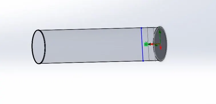
Simulations are carried out for flow of water through a pipe of internal radius 2.5cm and length 20cm. The boundary conditions are as follows:

1. Inlet - Velocity boundary condition

2. Outlet - Static Pressure boundary condition

3. Pipe Wall - Real wall boundary condition

We know that the Reynolds number for the flow is defined as:`Re = (rhoVD)/mu`

The density and viscosity values are fixed by the fluid properties and diameter is fixed by the geometry. So, Re depends only on the velocity.
Parametric study was carried out for 3 different inlet velocity and thus, for 3 different Reynolds numbers.

Mesh Independence Study

Before carrrying out the parametric study, a grid refinement study was performed to analyze the effect of grid size on the solution and find the optimum grid size for the problem.

The details for this study are shown below:

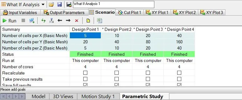
The velocity contours for the cut plane of the pipe along the flow for each grid size are as follows:

1. Design Point 1

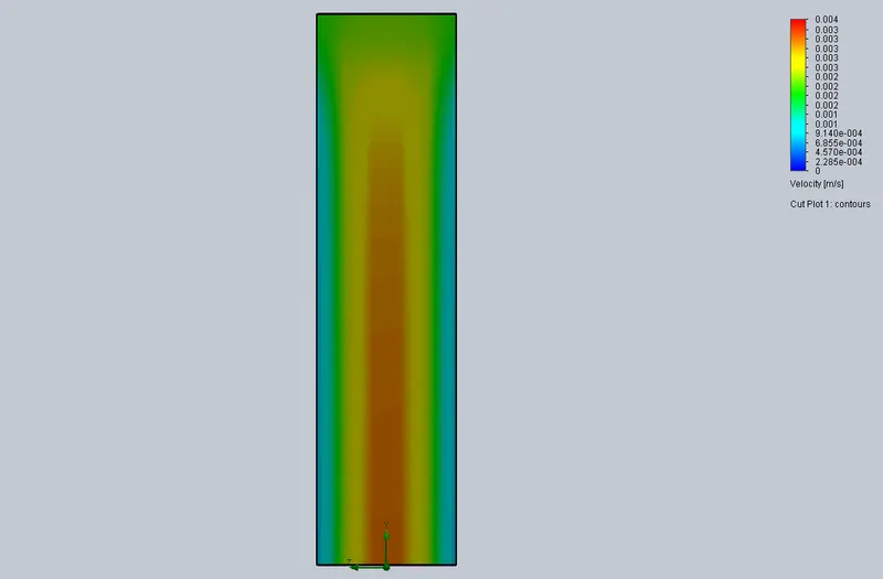
2. Design Point 2

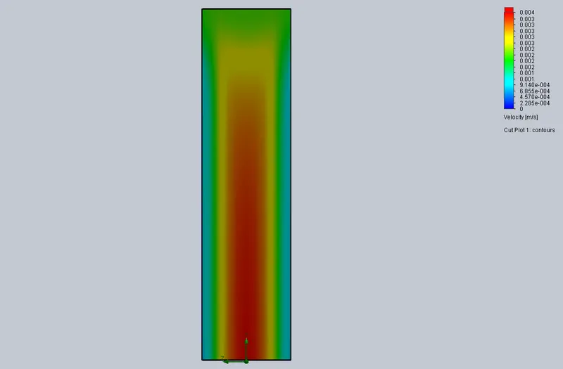
3. Design Point 3

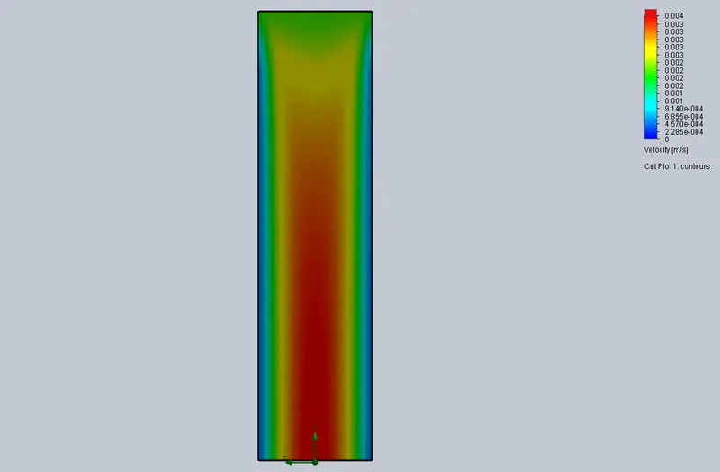
4. Design Point 4

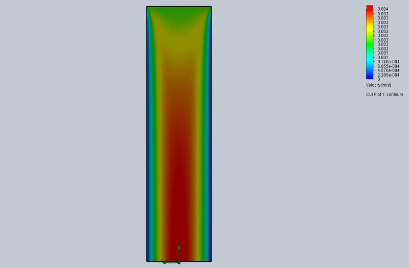
The velocity profile at a cross-section near the outlet of the flow for all grid sizes are shown below:

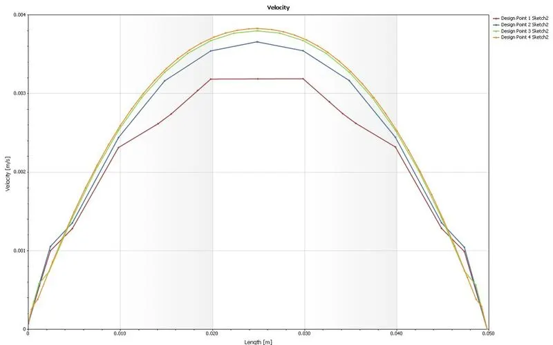
Now, we can clearly see from the plots that scenario 4 is much more accurate than scenarios 1 and 2. However, the difference between scenario 3 and 4 is not much pronounced. This implies that we have reached a reasonable accuracy, any further increase in grid size beyond that used in scenario 4 would be computationally expensive without any appreciable increase in accuracy of the solution. So, the scenario 4 is chosen as the optimum grid size for further simulations.

Effect of Reynolds number on the flow

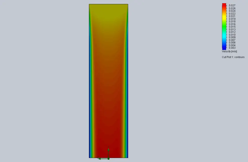
To study the effect of Re on the flow, the following different inlet velocities were taken; the velocity contours along a plane parallel to the direction of flow is also shown for each case.

1. u = 0.002 m/s, Re = 100

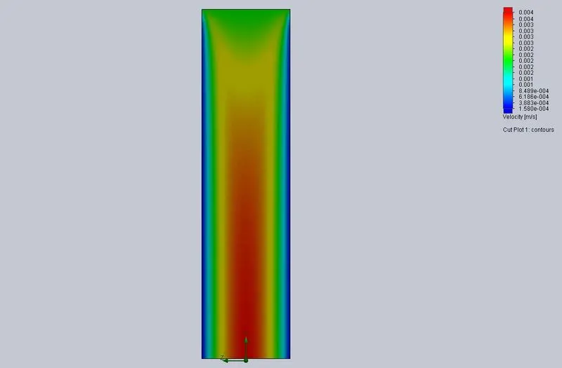
2. u = 0.02 m/s, Re = 1000

3. u = 0.2 m/s, Re = 10000

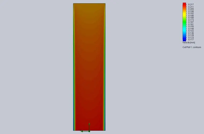
From the above velocity contours, we can see the boundary layer development in the flow. It should also be noted that for the first case, the length of the pipe is greater than the entrance length and hence the flow gets developed hydrodynamically. However, on increasing the Re, the entrance length increase and thus, for the other two case, the flow is still developing.

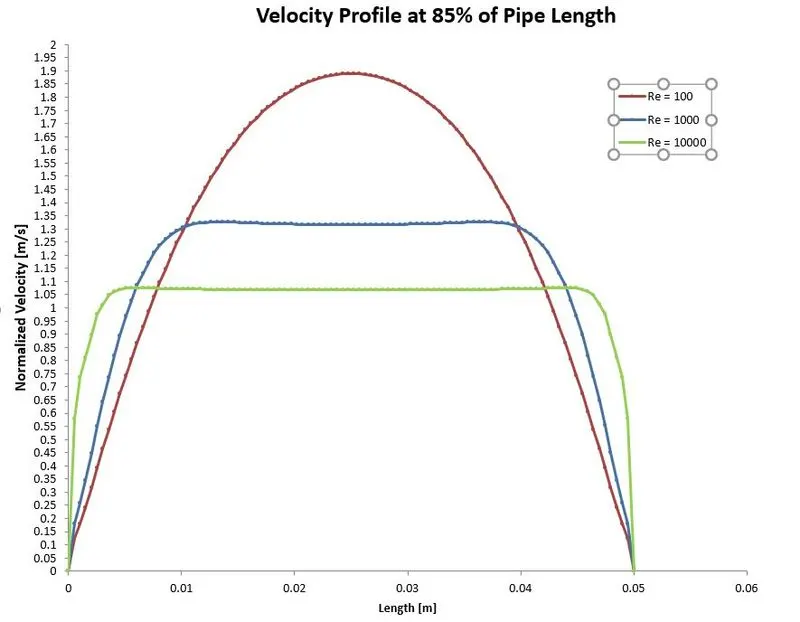
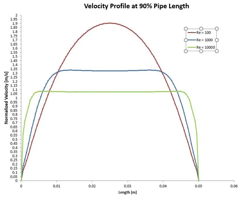
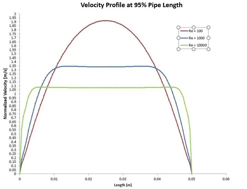
This effect can be better visualised by looking at the velocity profiles at different locations in the flow field. To make comparative analysis for the three cases simpler to analyze, the velocity has been non dimensionalised using the inlet velocity, so that the change in velocity can be better visualised and all the three cases have values in the same order of magnitude making comparision easier.

Analysis of the above plots:

1. It can be observed from the three plots that the flow in the 1st case has completely developed and hence there is no change in the velocity profile in the flow direction. The profile has assumed the Poiseuille Parabola shape. However, for the other 2 cases, the flow is still developing, and there exists a region in which there is no velocity gradient in the radial direction i.e., irrotational flow or flow external to the boundary layer. The length of this region is larger for the larger Re case. Moreover, along the flow direction, the profile is slowly evolving into the fully developed profile and the length of the irrotational flow region is decreasing.

2. It should also be noted that as Re increase, the length required for the flow to develop increases. The flow with higher Re will achieve the fully developed profile after travelling a longer distance in the flow direction. This is because with increasing Re, the boundary layer thickness decreases and thus, it would take more length for the boundary layer to become thick enough to cover the entire diamter or the pipe cross section. This effect can be visualised from the velocity contours shown above. For higher Re, the irrotational core remains in the flow domain for a longer pipe length compared to the lower Re flows. Moreover, higher the Re, more is the radius of this irrotational core.