Driver_model analysis using customised drive cycle
AIM-
Refer to below link for vehicle modelling using Simulink:
Prepare a new drive cycle excel file for the model and also include a hill-climbing angle to it. Revise the model file “Driver_Glider.slx” and comment on the results
Procedure-
After opening the model the files are saved in the directory and the model looks as-
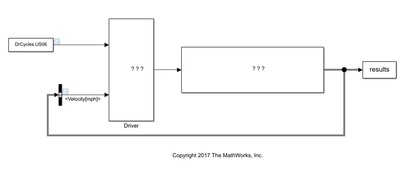
Output for standard drive cycle-
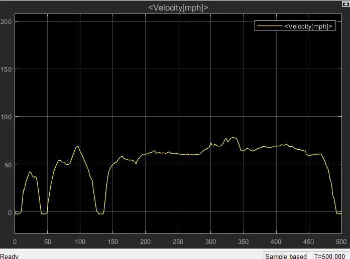
Here initially the input velocity cycle is Drcycles.US06 ,but we want to create our own drive cycle,for this purpose we create an excel sheet and create two columns in it ,one for time and one for velocity.This how a excel sheet looks.
Excel sheet-
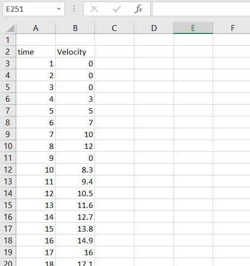
https://drive.google.com/file/d/1jyhwiNnCVSSlBKYltVQ3gEpUwZVuxzc9/view?usp=sharing
This is velocity cycle is created for 500 seconds
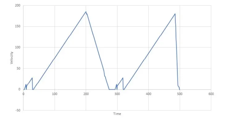
We need to import this excel data to workspace by using import data option so this data is imported using the name input_velocity.
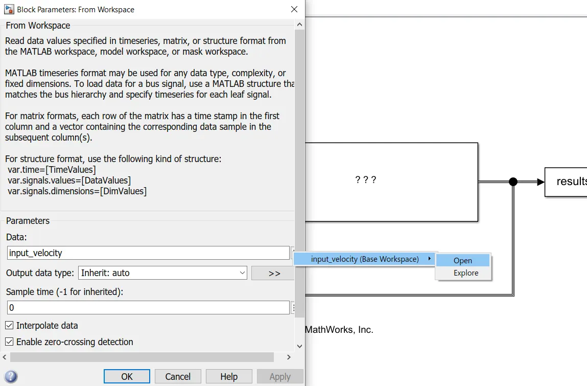
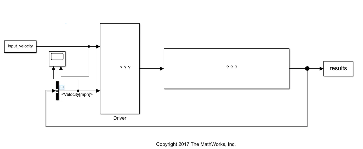
Now we add a block from work space and give it the name input_velocity and click from workspace as shown in below picture.so we have assigned our own input drive cycle
Model diagram-
Now we are also required to change the inclination angle theta in the grade force
After clicking on the subsystem the we click on the grade force to modify the parameters.
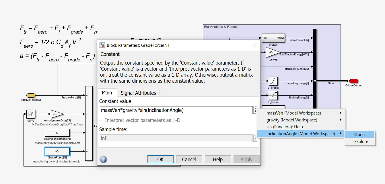
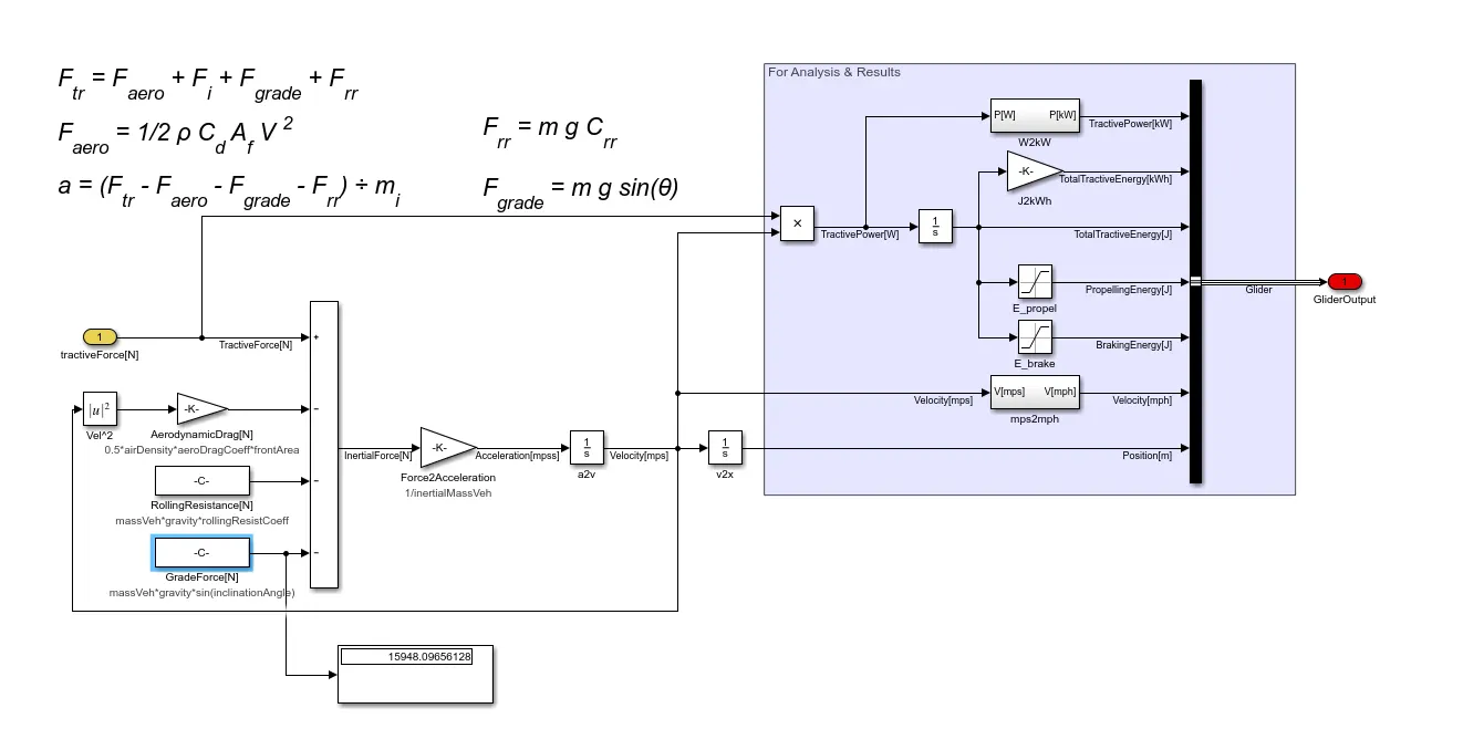
We want to change the inclination to 45 degrees ,so we enter its value in radians.If now we execute the model by adding a display block to grade force we get the hill climbing force.
OUTPUT-
Remarks-
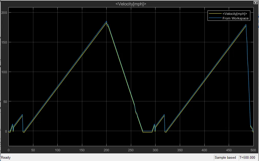
So as we increase the inclination angle the hill climbing force increases.
We can see the plotted graph between values from workspace which is in blue and output velocity values due to grade force which is in yellow.The hill climbing force is 15948 N.
Study 2-
AIM-
Model the WOT (Wide Open Throttle) response of GM EV1 car. Compare it with the official figures of the performance of a real vehicle. Prepare a table showing variation in acceleration time with a 5% change in vehicle parameters.
Introduction-
Wide open throttle (WOT) refers to an IC engine's maximum intake of air and fuel that occurs when the throttle plates inside the carburetor or throttle body are "wide open", providing the least resistance to the incoming air.
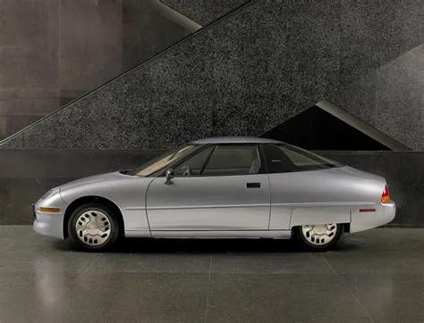
Specifications of GM EV1 car-
- Vehicle mass - 1400 kg^2
- Drag coefficient - 0.19
- Rolling resistance - 0.0048
- Tyre radius - 0.30 m
- Gear ratio G = 11
- Frontal area = 1.8 m^2
- Tmax = 140Nm and ωc = 733 rad s−1, note this means T = Tmax until v = 19.8ms−1 (= 71.3 kph);
- Above 19.8ms−1 the motor operates at a constant 102 kW
- vmax = 35.8 m/sec
Solution-
For vehicle on ground the traction force Fte
Fte = μrr*m*g + 0.625*A*Cd*ν^2 + m*a + I*G^2*a/ηg*r^2
we know acceleration is change in velocity
G*r/T =μrr*m*g + 0.625*A*Cd*ν^2 + (m + I*G^2/ηg*r^2)* dv/dt
In initial acceleration phase T = Tmax ,the equation becomes
G*r/Tmax =μrr*m*g + 0.625*A*Cd*ν^2 + (m + I*G^2/ηg*r^2)* dv/dt
By increasing the mass by 5% we can compensate the term force due to angular acceleration .
Total mass = mass of vehicle + mass of passenges + 5 % of mass = 1540kg.
Now putting all parameters in the above equation we get
0.95 × 37 × 140 = 72.4 + 0.214v^2 + 1560*dv/dt
So
dv/dt = 3.11 − 0.000137*v^2 ------------------(1)
Once speed reached 19 m/s then we need to replace T we have T = 102000/ 37*V
0.95 × 37 × 2756/v= 72.4 + 0.214v2 + 1560* dv/dt
dv/dt = 62.1/v− 0.046 − 0.000137*v^2---------(2)
For calclating the variation of velocity we need to use Matlab or excel .
We need to write this differential so that it can be written as a code
we can understand that dv/dt is change in velocity during time interval dt ,we can write dv = Vn+1 - Vn , dt is small time interval we replace equation 1 and 2 as -
Vn+1 = Vn + dt(3.11 - 0.000137*Vn^2) -------(3)
Vn+1= Vn + dt(62.1/Vn-0.0046-0.000137*Vn^2)------(4)
Matlab code -
t=linspace(0,50,501); % 0 to 50 s, in 0.1 s steps
vel=zeros(1,501); % 501 readings of velocity
d=zeros(1,501);% Array for storing distance traveled
dT=0.1; % 0.1 second time step
for n= 1:500
% Now follow equations 7.17 & 7.18
if  vel(n)<19.8 % Torque constant till this point
    vel(n+1) = vel(n) + dT*(3.11 - (0.000137*(vel(n)^2)));
elseif vel(n)>=35.8
        vel(n+1)= vel(n)
else
vel(n+1)=vel(n)+dT*(62.1/vel(n)-(0.046)-(0.000137*(vel(n)^2)));
   end;
d(n+1)=d(n) + 0.1*vel(n); % Compute distance traveled.
end;
vel=vel.*3.6; % Multiply by 3.6 to convert m/sec to kph
plot(t,vel)
hold on
axis([0 20 0 150]);
xlabel("Time/seconds");
ylabel("Velocity/kph");
title("Full power (WOT) acceleration of electric scooter")
Output-
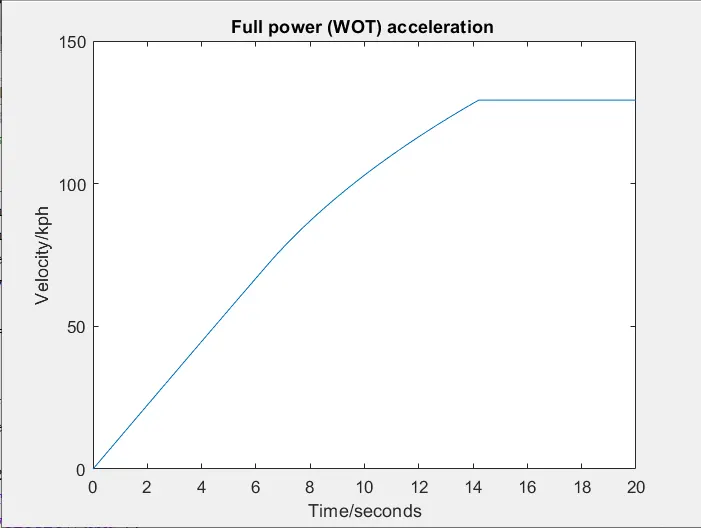
Comparision with standard website data-
Now if we want to compare our caluclation with standard website
https://en.wikipedia.org/wiki/General_Motors_EV
- From website the we get the time taken by the vehicle to reach from 0 to 60 kmph i.e 26.94 m/s is 8sec.
- Now if we include new lines in the code to see the time where the vehicle attains maximum speed and also the velocity at t = 8seconds we can compare our model with the standard model.
Program code-
t=linspace(0,50,501); % 0 to 50 s, in 0.1 s steps
vel=zeros(1,501); % 501 readings of velocity
d=zeros(1,501);% Array for storing distance traveled
dT=0.1; % 0.1 second time step
for n= 1:500
% Now follow equations 7.17 & 7.18
if  vel(n)<19.8 % Torque constant till this point
    vel(n+1) = vel(n) + dT*(3.11 - (0.000137*(vel(n)^2)));
elseif vel(n)>=35.8
        vel(n+1)= vel(n);
else
vel(n+1)=vel(n)+dT*(62.1/vel(n)-(0.046)-(0.000137*(vel(n)^2)));
   end;
d(n+1)=d(n) + 0.1*vel(n); % Compute distance traveled.
end;

for n= 1:(length(t-1))
    if vel(n+1)==vel(n)
        fprintf('the time to attain maximum velocity is')
        display (t(n));
        break;
    end
end
 for n=1:(length(t-1))
     if t(n)== 8
         fprintf('At time = 8seconds the velocity is')
         display (vel(n))
     end
 end
vel=vel.*3.6; % Multiply by 3.6 to convert m/sec to kph
plot(t,vel)
axis([0 20 0 150]);
xlabel("Time/seconds");
ylabel("Velocity/kph");
title("Full power (WOT) acceleration of electric scooter")
Output-

Our model at t = 8 seconds the speed is 24.1622m/s but in standard data when t= 8 seconds the speed is 26.94m/s,so here the variation is not very large considering the assumptions and simplified system we have taken.
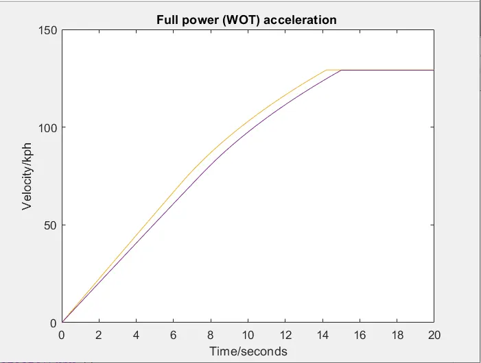
Variation in parameters for 5 % change in vehicle parameters-
Vehicle mass =1617 Kgs
μrr = 0.0048
Frontal area = 1.8 m^2
Tire radius = 0.315m
Tmax = 140N
now the equations (1) and (2) change as
Vn+1 = Vn + dt(2.83 - 0.000130*Vn^2) -------(3)
Vn+1= Vn + dt(59.51/Vn-0.00474-0.000130*Vn^2)------(4)
Writing the matlab code to compare the two cases
Matlab code-
t=linspace(0,50,501); % 0 to 50 s, in 0.1 s steps
vel=zeros(1,501); % 501 readings of velocity
d=zeros(1,501);% Array for storing distance traveled
dT=0.1; % 0.1 second time step
for n= 1:500
% Now follow equations 7.17 & 7.18
if  vel(n)<19.8 % Torque constant till this point
    vel(n+1) = vel(n) + dT*(3.11 - (0.000137*(vel(n)^2)));
elseif vel(n)>=35.8
        vel(n+1)= vel(n);
else
vel(n+1)=vel(n)+dT*((62.1/vel(n))-(0.046)-(0.000137*(vel(n)^2)));
   end;
end;
vel=vel.*3.6; % Multiply by 3.6 to convert m/sec to kph
plot(t,vel)
hold on
axis([0 20 0 150]);
xlabel("Time/seconds");
ylabel("Velocity/kph");
title("Full power (WOT) acceleration of electric scooter")
for n = 1:500
if  vel(n)<20.99 % Torque constant till this point
    vel(n+1) = vel(n) +dT*(2.83 - (0.000130* (vel(n)^2)));
elseif vel(n)>=35.8
        vel(n+1)= vel(n);
else
vel(n+1)= vel(n) + dT*((59.51/vel(n))-0.00474-0.000130*vel(n)^2);
   end;
end
 vel=vel.*3.6; % Multiply by 3.6 to convert m/sec to kph
 plot(t,vel)
axis([0 20 0 150]);
xlabel("Time/seconds");
ylabel("Velocity/kph");
title("Full power (WOT) acceleration of electric scooter")
Output-
Link to comparision excel file -
https://drive.google.com/file/d/1AMvLJxfuQTTaLvJ_MdKj3hG5am3c_yUj/view?usp=sharing