Discretization basics for range of dx

OBJECTIVE: TO WRITE A PROGRAM TO COMPARE THE FIRST, SECOND, AND FOURTH ORDER APPROXIMATIONS OF THE FIRST DERIVATIVE WITH ANALYTICAL DERIVATIVE WHEN THE VALUE OF dx IS VARYING.

Given function: `sin x/x^3` at `x=pi/3`

Answer:

For calculating the first, second and fourth order approximation, functions of each order are made and called in the main function.

First Order Approximation Function Code:

function first_order_error= first_order_approximation(x,dx)
  
 %function sin(x)/x^3
 %analytical_derivative=(cos(x)*x^3 - sin(x)*3*x^2)/x^6
 analytical_derivative=(cos(x)*x^3 - sin(x)*3*x^2)/x^6;

 %first order approximation 
 forward_differencing= ((sin(x+dx)/(x+dx)^3)-(sin(x)/x^3))/dx;

 first_order_error = abs(forward_differencing-analytical_derivative);

 endfunction
 

Here we can see that a function named first_order_approximation is defined.

In the 5th line, the analytical derivative of the given function i.e `sin x/x^3` is calculated.

After that, the first-order approximation or forward differencing is calculated. At the end, the absolute error is calculated.

Second-Order Approximation Function Code:

%defining the function for secind order approximation
function second_order_error=second_order_approximation(x,dx)
 
 analytical_derivative=(cos(x)*x^3 - sin(x)*3*x^2)/x^6;

 central_differencing=((sin(x+dx)/(x+dx)^3)-(sin(x-dx)/(x-dx)^3))/(2*dx);

  second_order_error=abs(central_differencing-analytical_derivative);
endfunction

Similarly, the analytical derivative, central differencing or second-order approximation and absolute error are calculated.

Fourth-Order Approximation Code:

%defining the function for fourth order approximation
function fourth_order_error=fourth_order_approximation(x,dx)
 
 analytical_derivative=(cos(x)*x^3 - sin(x)*3*x^2)/x^6;

 fourth_order_differencing=((sin(x-2*dx)/(x-2*dx)^3)-(8*(sin(x-dx))/(x-dx)^3)+(8*(sin(x+dx))/(x+dx)^3)-(sin(x+2*dx)/(x+2*dx)^3))/(12*dx);

  fourth_order_error=abs(fourth_order_differencing-analytical_derivative);
endfunction

As all the functions are defined, now the main function is made.

1. The input value of each function is x and dx, so they must be defined before calling out the function.
2. The value of dx is between `pi/4 and pi/400` in which 20 equidistant points are present.
3. For each value of dx, first, second, and fourth order errors are calculted.
4. For each value of dx, all three functions are called to give an output of errors.

After calculating the errors, the graph is being plotted between dx and error(s).

clear all
close all
clc

%given value of x
x=pi/3;

%declaring the range or matrix of the dx
dx=linspace(pi/4,pi/400,20);

for i=1:length(dx)
  first_order_error(i)= first_order_approximation(x,dx(i));
  second_order_error(i)= second_order_approximation(x,dx(i));
  fourth_order_error(i)= fourth_order_approximation(x,dx(i));
endfor

%ploting of errors and dx in the same graph
figure(1)
%using loglog command for larger graph view
loglog(dx,first_order_error,'b')
hold on
loglog(dx,second_order_error,'r')
hold on
loglog(dx,fourth_order_error,'g')
xlabel('dx')
ylabel('errors')
legend('first order error','second order error','fourth order error')

The output of the code is:

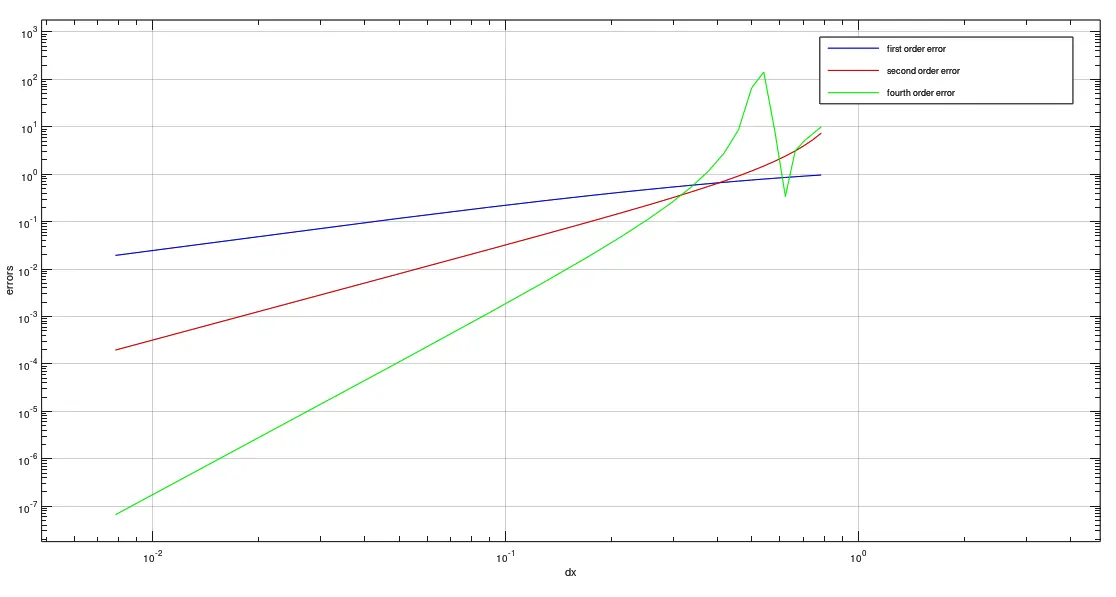
From the above plot, the following Conclusions are made:

1. In the first-order approximation, when the value of dx decreases the value of errors also decreases with some rate smaller than second and fourth order approximation. This is because the terms from which we are neglecting while deriving the formulae is of first order.
2. In second order approximation, on decreasing the value of dx the value of errors also decreases with a much greater slope than that of first order approximation. the reason behind it is that, the terms from which the we neglect are of second order hence the name second order approximation.
3. In fourth order approximation, on decreasing the value of dx the value of errors also decreases. and the slope of the plot is much greater than the two plots.

Slope calculating code:

%slope calculations
clear all 
close all
clc
%slope=(y2-y1)/(x2-x1)

%first order error slope
p1=[0.78177 0.98815]; %end points of the curve in blue  
p2=[0.0078569 0.019823];
slope_first_order=(p2(2)-p1(2))/(p2(1)-p1(1))

%second order error slope
p3=[0.78177 7.4134]; %endpoints of the curve in red
p4=[0.0078569 0.00020149];
slope_second_order=(p4(2)-p3(2))/(p4(1)-p3(1))

%fourth order error slope
p5=[0.78177 10.165];
p6=[0.0078569 6.841*e^-8];
slope_fourth_order=(p6(2)-p5(2))/(p6(1)-p5(1))

Here the points are selected from the plot of above code.

The output of the code is :

slope_first_order =  1.2512
slope_second_order =  9.5789
slope_fourth_order =  13.132
>>

From here we can compare the slope of the curves.

It is clear here that the on small dx, the fourth order approximation gives the least error while calculating the first order derivative.