3D transient CFD analysis of cyclone separator for prediction of its collection efficiency.
Aim – Three dimensional transient CFD study for prediction of collection efficiency of a cyclone separator.
Introduction –
Cyclone separators or simply cyclones are separation devices (dry scrubbers) that use the principle of inertia to remove particulate matter from flue gases.
A high speed rotating (air) flow is established within a cylindrical or conical container called a cyclone. Air flows in a spiral pattern, beginning at the top (wide end) of the cyclone and ending at the bottom (narrow) end before exiting the cyclone in a straight stream through the center of the cyclone and out the top. Larger (denser) particles in the rotating stream have too much inertia to follow the tight curve of the stream and strike the outside wall, falling then to the bottom of the cyclone where they can be removed. In a conical system, as the rotating flow moves towards the narrow end of the cyclone the rotational radius of the stream is reduced, separating smaller and smaller particles. They can reach efficiencies up to 99% for particles greater than 5 μm. They are widely used in the oil industry, cement industry, thermal power plants etc.
From the design point of view, engineers are mainly concerned with the collection efficiency and pressure drop across the separator. CFD has great applications in predicting these parameters essential for a good design.
Several empirical models are also available to predict the collection efficiency. A brief description of some of these are–
- Lapple - Lapple model (1951) was developed based on force balance without considering the flow resistance. Lapple assumed that a particle entering the cyclone is evenly distributed across the inlet opening.
- Koch and Licht - Koch and Licht (1977) collection theory recognized the inherently turbulent nature of cyclones and the distribution of gas residence times within the cyclone. Koch and Licht described particle motion in the entry and collection regions with the additional following assumptions:
- The tangential velocity of a particle is equal to the tangential velocity of the gas flow, i.e. there is no slip in the tangential direction between the particle and the gas.
- The tangential velocity is related to the radius of cyclone by:
uRn = constant.
- Li and Wang – The Li and Wang (1989) model includes particle bounce or re-entrainment and turbulent diffusion at the cyclone wall. A two-dimensional analytical expression of particle distribution in the cyclone was obtained.
- Iozia and Leith - Iozia and Leith (1990) logistic model is a modified version of Barth (1956) model which is developed based on force balance. The model assumes that a particle carried by the vortex endures the influence of two forces: a centrifugal force and a flow resistance.
Modelling and Solving approach –
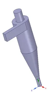
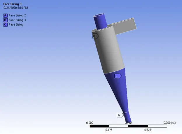
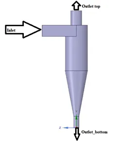
Solid Model – A 3D model of cyclone separator setup was already provided. Volume extraction feature (using edge selection) was employed to extract the fluid volume. The geometry was then exported to Ansys Mesher. The image of the model in Spaceclaim is provided below –
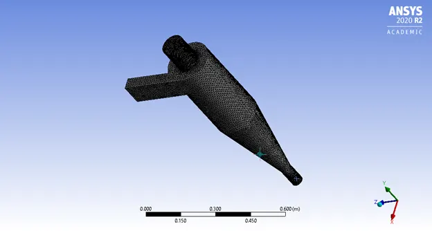
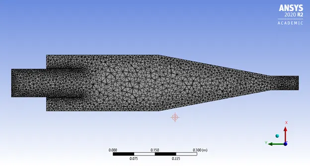
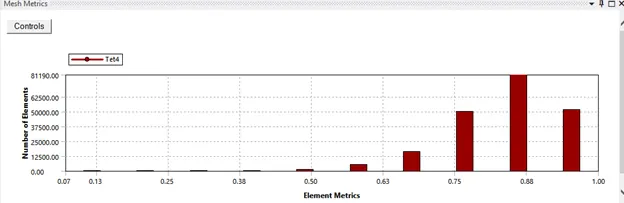
Meshing – Tetrahedral mesh has been utilized to mesh the 3D geometry with a global element size of 10 mm. Apart from this, face sizing controls at different faces as given in the below table have been utilized to create a suitable mesh.
|
Method |
Tetrahedral |
|
Global Element size |
10 mm |
|
Capture curvature |
No |
|
Capture Proximity |
No |
|
Face Sizing 2 (A) |
5 mm |
|
Face Sizing 3 (B) |
5 mm |
|
Face Sizing (C) |
10 mm |
|
Number of elements |
205092 |
|
Element quality (Min/Max/Avg./ Std. Deviation) |
0.07/1.00/0.84/0.00945 |
Solver Settings – Ansys Fluent was used as the solver and steady state simulations have been performed using a pressure based solver.
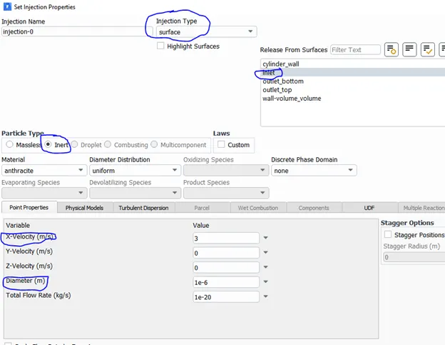
Boundary conditions and materials – Anthracite has been used as the inert material injected along with air.
The named selections are mentioned in the below figure. Inlet air velocity and particle velocity have been kept as the same during the simulations. Apart from the general boundary conditions, the boundary conditions for the Discrete Phase Method (DPM) also need to be specified for the problem. The boundary conditions assigned to these named selections are in the below table-
|
Named Selection |
Boundary condition (DPM type) |
|
Inlet |
Velocity inlet (Reflect) |
|
Cylinder wall |
Wall(Reflect) |
|
Outlet_top |
Pressure outlet (Escape) |
|
Outlet_bottom |
Pressure Outlet (Trap) |
Reflect - It refelcts the particle from the boundary selected. The coefficient of restitution is given in normal aand tangential direction. The normal direction e is given as
`e_n = v_(2,n)/v_(2,n)`
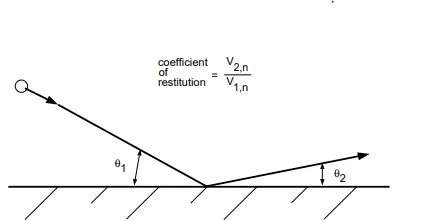
A normal or tangential coefficient of restitution equal to 1.0 implies that the particle retains all of its normal or tangential momentum
after the rebound (an elastic collision). A normal or tangential coefficient of restitution equal to 0.0 implies that the particle retains
none of its normal or tangential momentum after the rebound. Non-constant coefficients of restitution can be specified for wall zones with the “reflect” type boundary condition. The coefficients are set as a function of the impact angle `theta_1`. The default values of `e_n`and `e_t` is 1.0,
Escape - It reports the particle as having “escaped” when it encounters the boundary in question. Trajectory calculations are terminated.
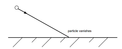
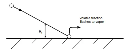
Trap - It terminates the trajectory calculations and records the fate of the particle as “trapped”. In the case of evaporating droplets, their entire mass instantaneously passes into the vapor phase and enters the cell adjacent to the boundary.In the case of combusting particles, the remaining volatile mass is passed into the vapor phase.
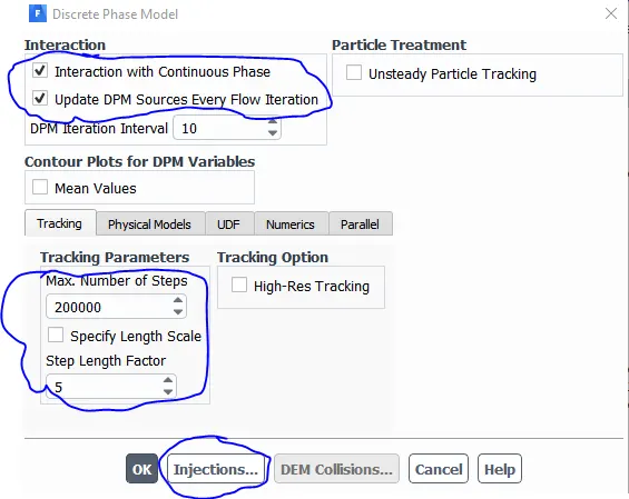
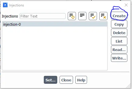
Computational model – RNG k -epsilon (standard wall function, swirl dominated flow) along with DPM model have been used for the simulations. Also, gravitational acceleration in the y direction is specified as -9.81 m/s2. The detailed procedure for setting up the DPM model has been highlighted in the below figures. It must be noted that the DPM model dialogue box shared below is used only for setting up the DPM model and the injection particle parameters. The other boundary conditions must be setup in the boundary condition tab available.
The solution setup is now complete.
Spatial Discretization – Coupled Pressure velocity coupling scheme was used to solve the Navier Stokes Equations. The default solution controls and methods have been used.
|
Gradient |
Least Squares Cell Based |
|
Pressure |
Second Order |
|
Momentum |
Second Order Upwind |
|
Turbulent kinetic energy |
Second order upwind |
|
Turbulent dissipation rate |
Second order upwind |
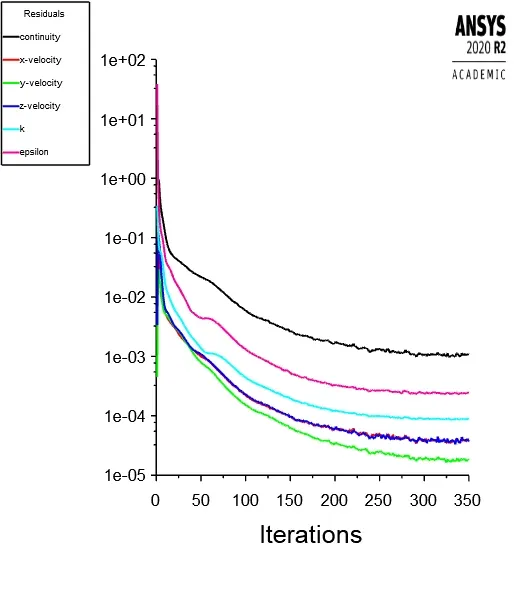
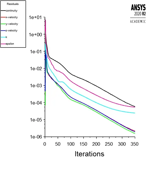
The solution has been initialized using the Standard Initialization method (from inlet) and has been run for 300 iterations for case 1 and 350 iterations for case 2.
|
Case 1 |
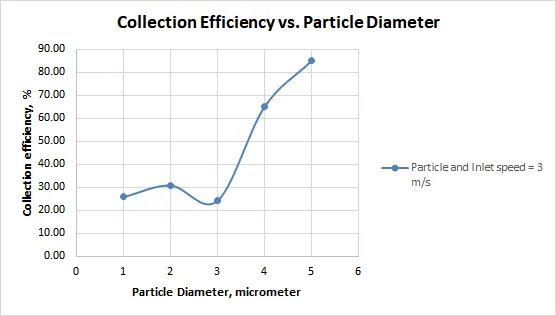
Constant velocity (both anthracite and air 3 m/s) – Particle diameter varied from 1 to 5 micrometers |
|
Case 2 |
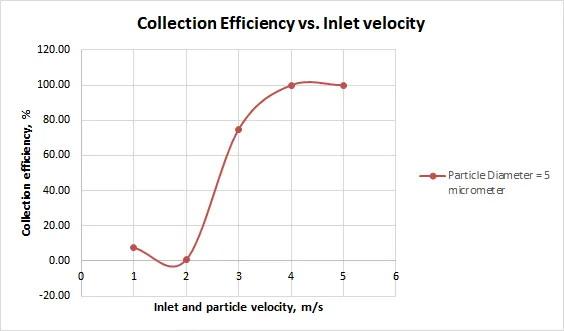
Constant particle diameter (5 micrometer) – Particle and air velocity varied from 1 to 5 m/s. |
Results and Discussions
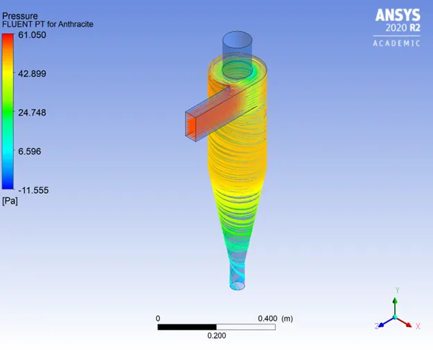
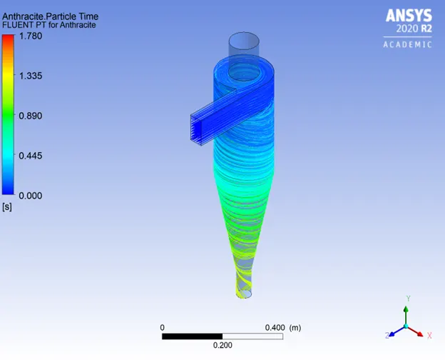
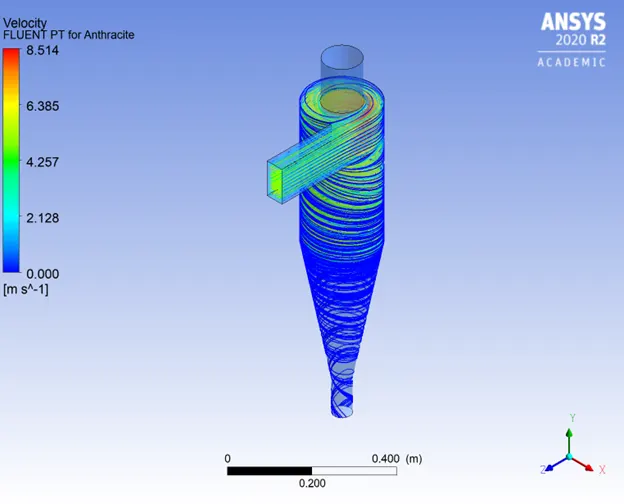
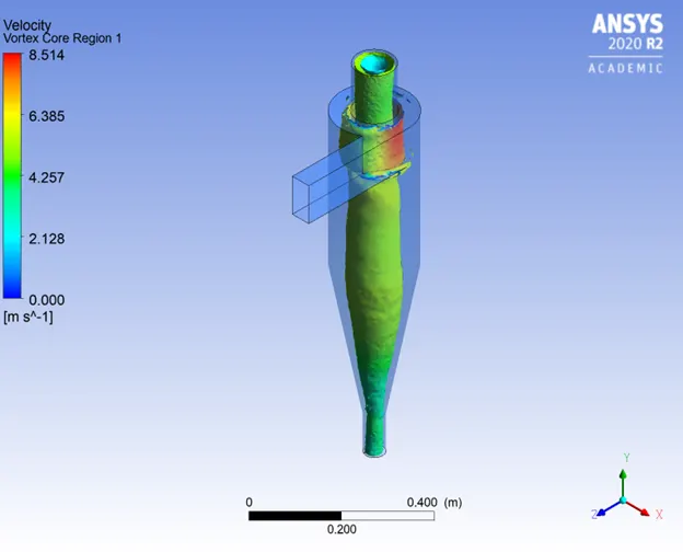
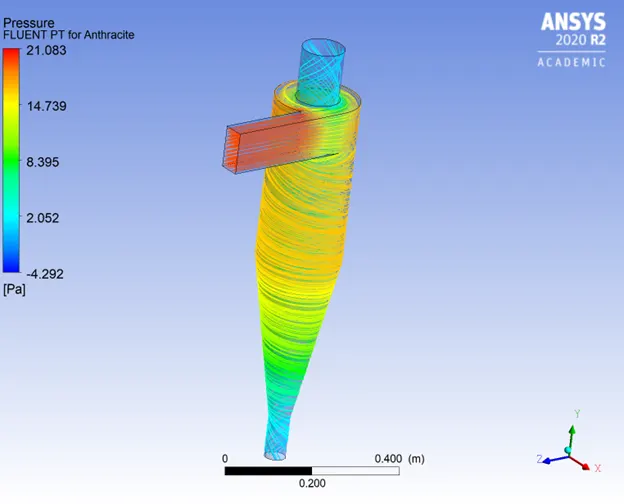
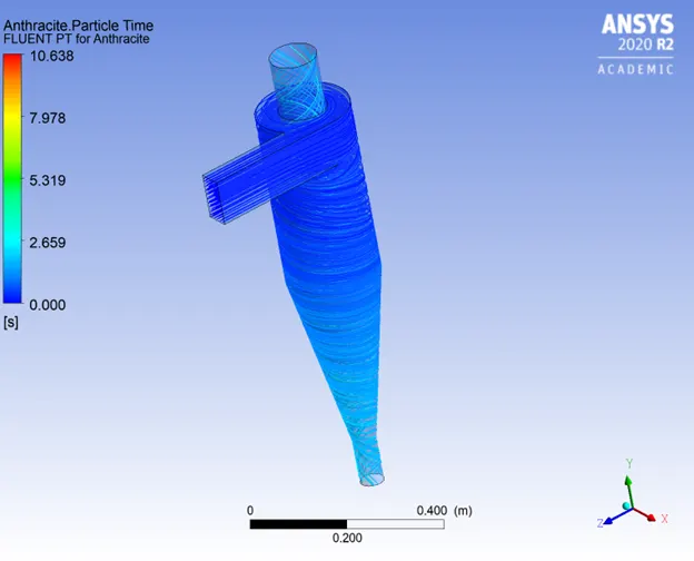
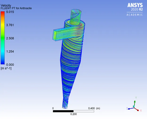
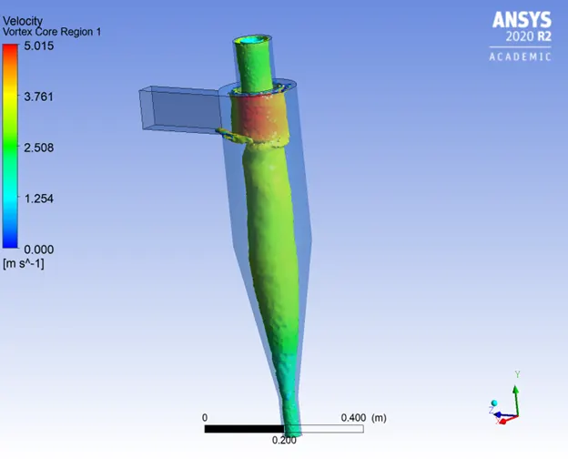
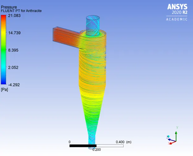
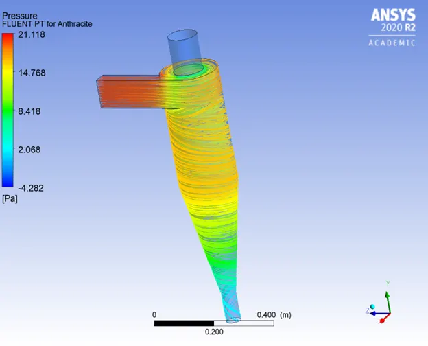
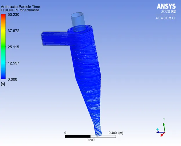
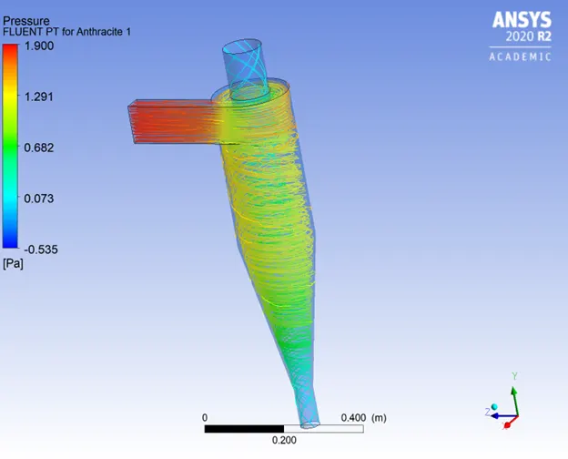
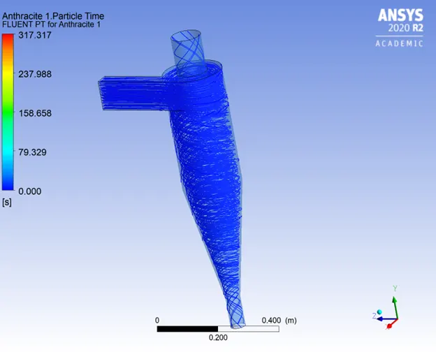
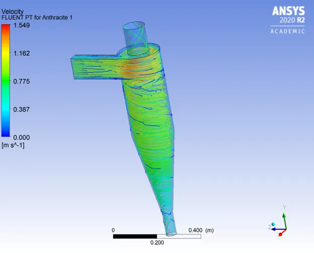
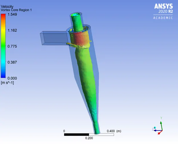
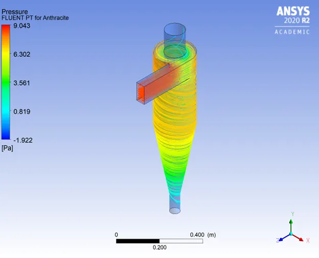
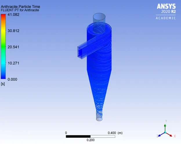
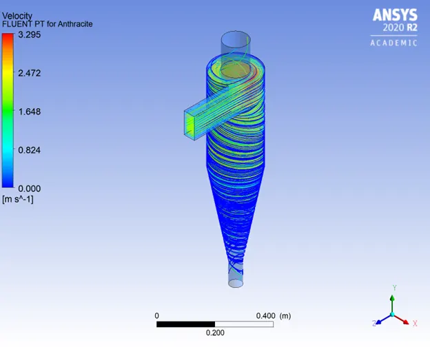
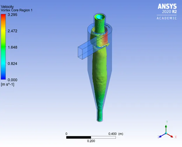
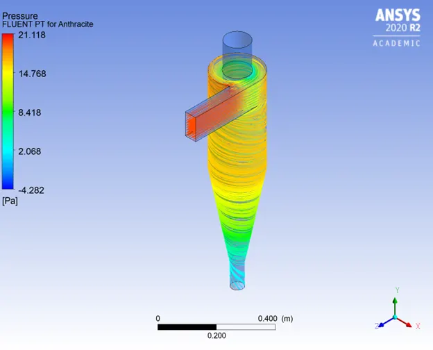
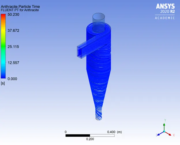
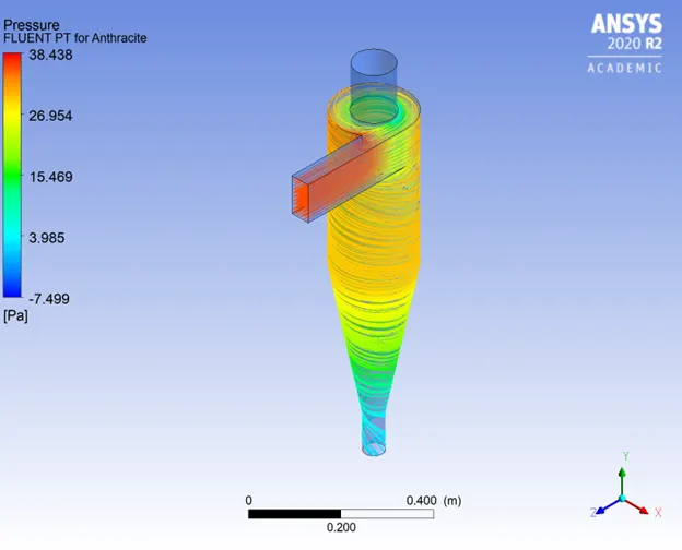
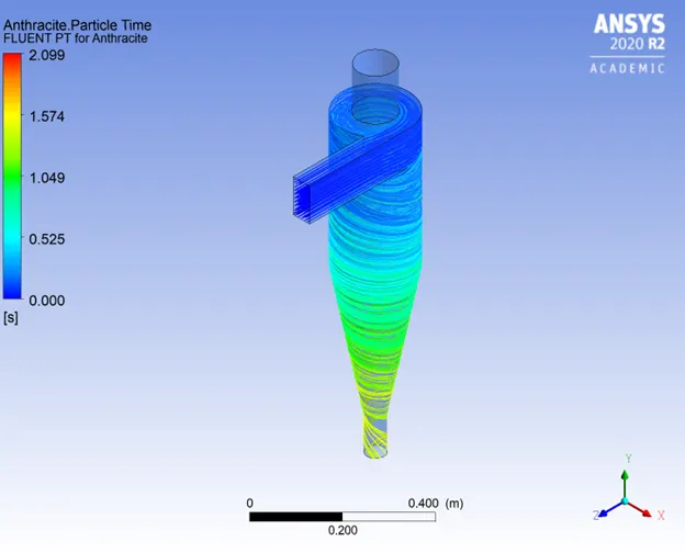
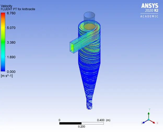
The graphical representation of collection efficiency for the two cases clearly verifies the fact that collection efficiency is directly proportional to the particle size and flow (or particle) velocity. This is because increase in either the mass or the velocity the centrifugal forces increase and more particles hit the cyclone wall and are collected at the bottom. The other important pressure and velocity contours highlighting the flow phenomenon for both the cases have been shown here. Collection efficiency is given as -
`η=(Trapped)/(Total)*100`
It can also be inferred from the below table that the pressure drop is directly proportional to the velocity of flow. It doesn’t depend on the particle size as such small particles have negligible interaction with the flow.
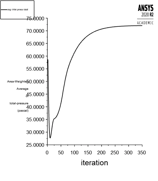
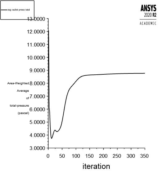
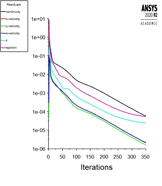
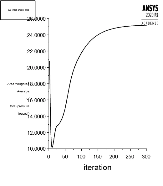
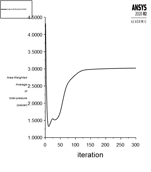
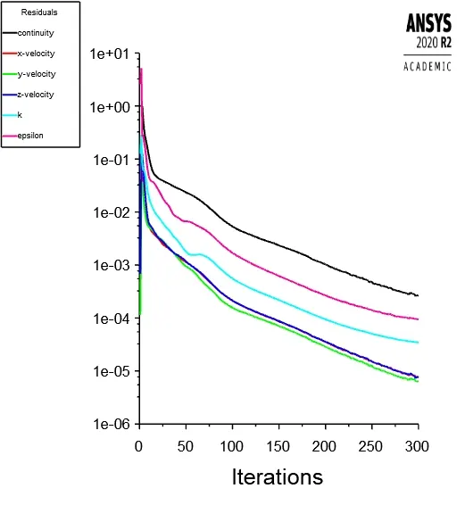
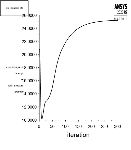
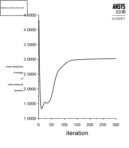
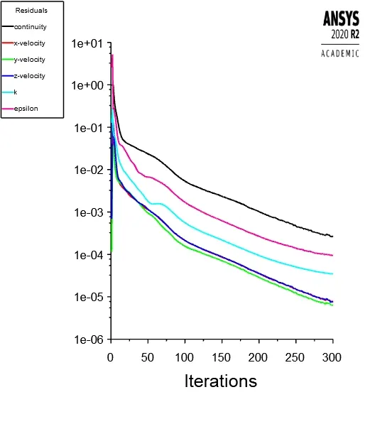
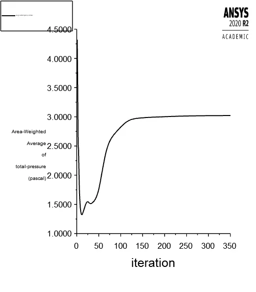
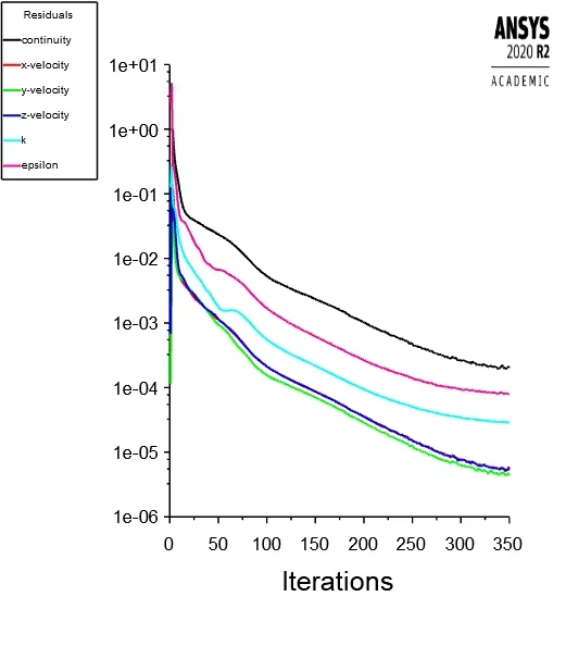
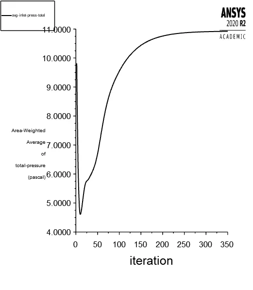
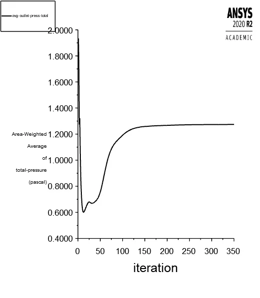
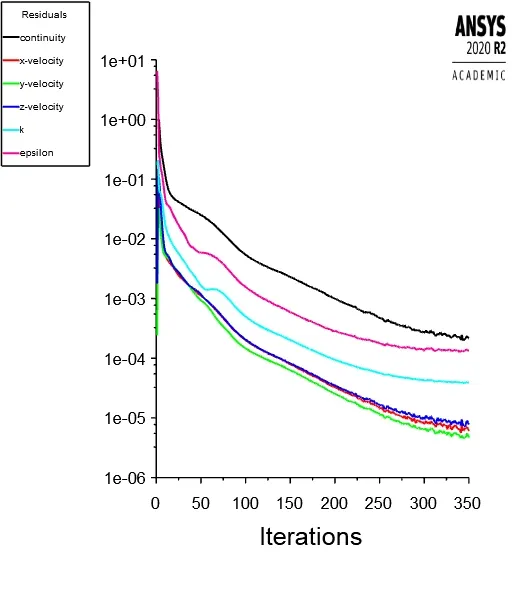
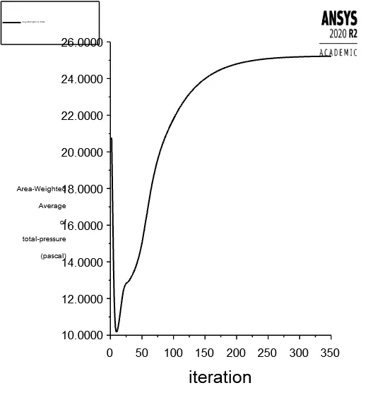
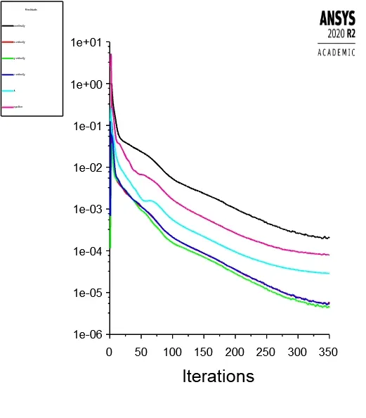
To check for convergence, in addition to residuals, average total pressures at the inlet at top outlet have also been considered. The solution has been considered to be converged only after the pressure changes become negligible and residuals reach below 1e-03.
CASE 1
| Inlet and Particle velocity (m/s) |
Particle Diameter (micrometer) |
Number of iterations | Total | Escaped | Trapped | Incomplete | Pressure drop (Pa) |
Collection Efficiency |
Mass conservation |
| 3 | 1 | 300 | 120 | 25 | 31 | 64 | 22.167 | 25.83 | 8.9E-07 |
| 2 | 300 | 120 | 16 | 37 | 67 | 22.167 | 30.83 | 8.9E-07 | |
| 3 | 300 | 120 | 9 | 29 | 82 | 22.167 | 24.17 | 1.8E-07 | |
| 4 | 300 | 120 | 2 | 78 | 40 | 22.167 | 65.00 | 8.9E-07 | |
| 5 | 300 | 120 | 0 | 102 | 18 | 22.167 | 85.00 | 4.3E-07 | |
| CASE 2 | |||||||||
| Particle Diameter (micrometer) |
Inlet and Particle velocity (m/s) |
Number of iterations | Total | Escaped | Trapped | Incomplete | Pressure drop (Pa) |
Collection Efficiency |
Mass Conservation |
| 5 | 1 | 350 | 120 | 8 | 9 | 103 | 2.169 | 7.50 | 1E-07 |
| 2 | 350 | 120 | 2 | 1 | 117 | 9.646 | 0.83 | 8E-08 | |
| 3 | 350 | 120 | 0 | 90 | 30 | 22.199 | 75.00 | 4.3E-07 | |
| 4 | 350 | 120 | 0 | 120 | 0 | 40.071 | 100.00 | 3.8E-07 | |
| 5 | 350 | 120 | 0 | 120 | 0 | 63.281 | 100.00 | 6.9E-07 |
CASE 1 –
Particle size = 1 micrometer
Particle size = 2 micrometer
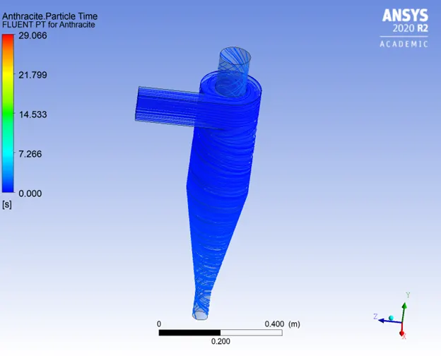
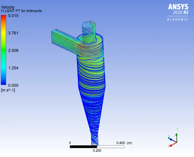
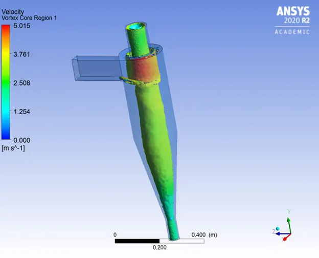
Particle size = 3 micrometer
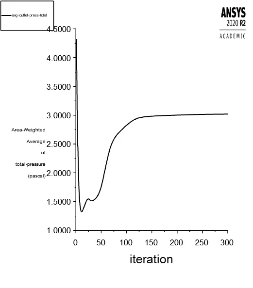
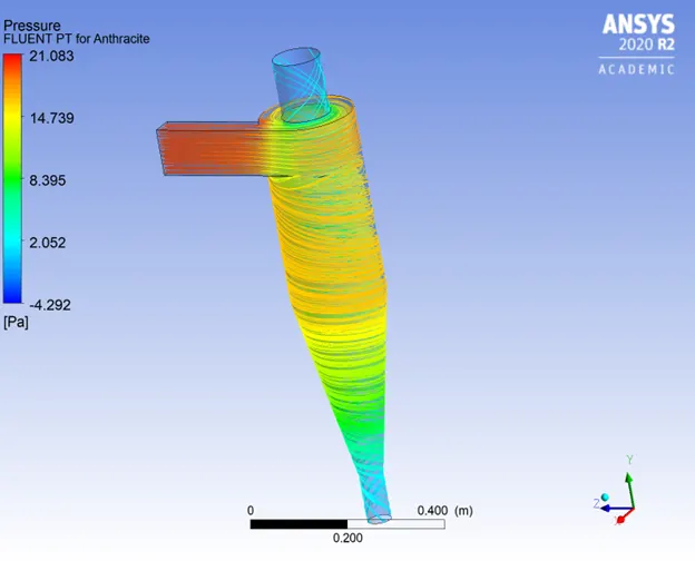
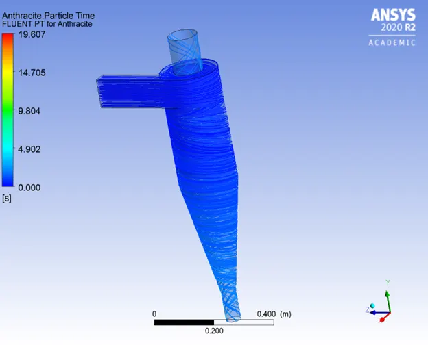
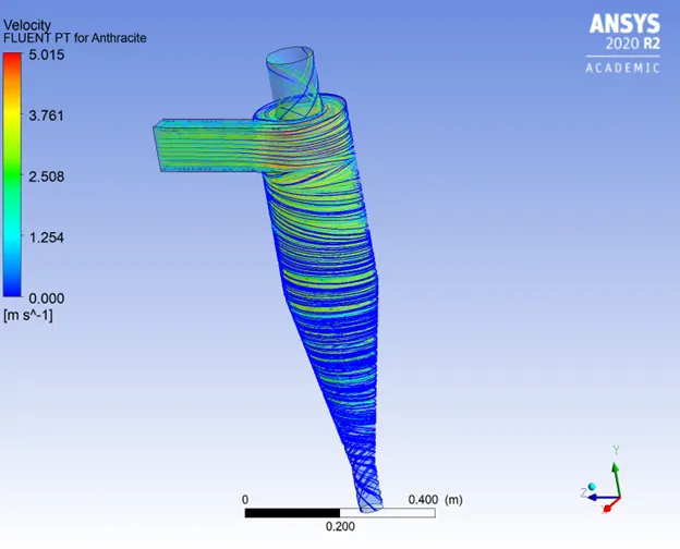
Particle size = 4 micrometer
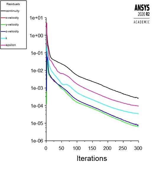
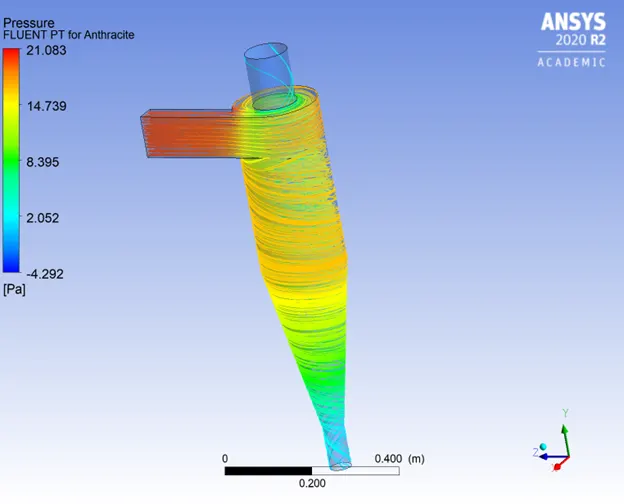
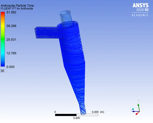
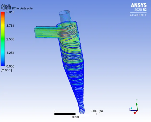
Particle size = 5 micrometer
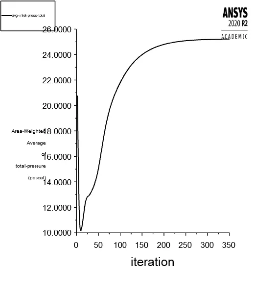
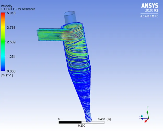
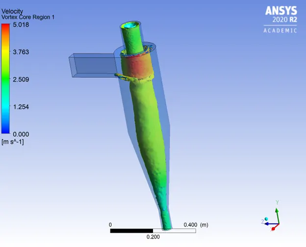
CASE 2
Velocity = 1 m/s
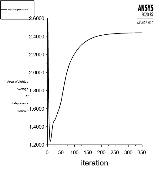
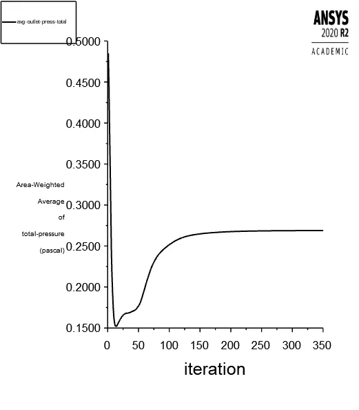
Particle velocity = 2 m/s
Particle velocity = 3 m/s
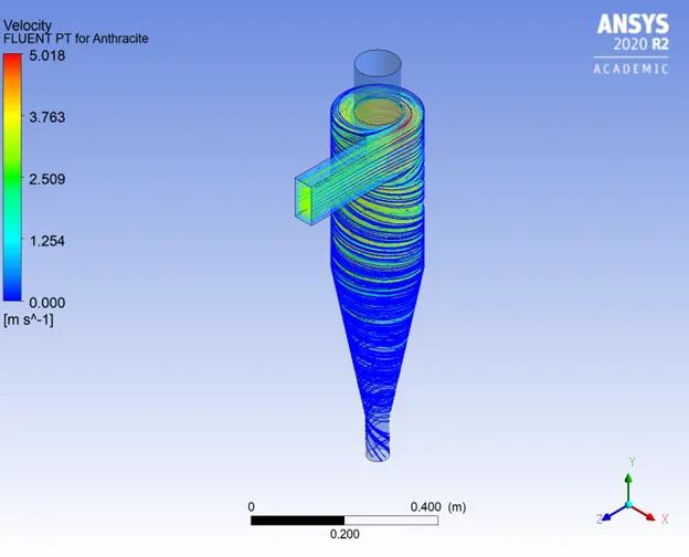
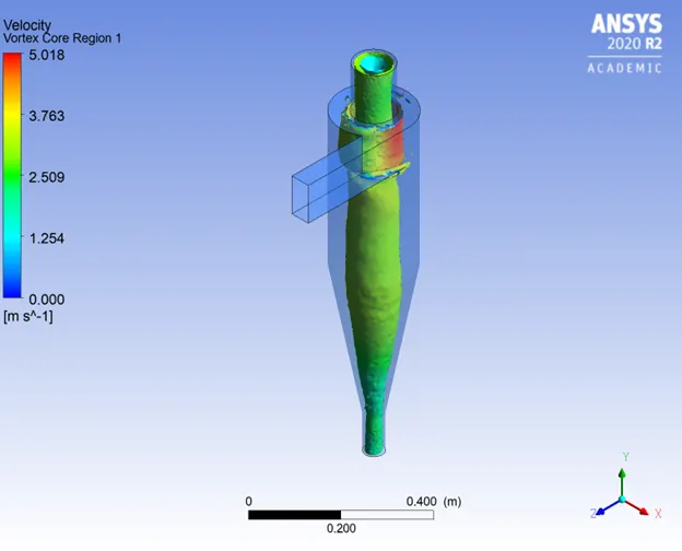
Particle velocity = 4 m/s
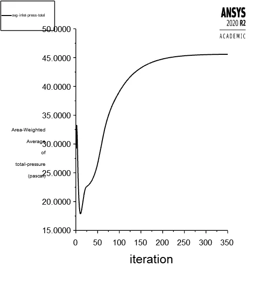
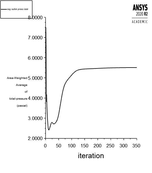
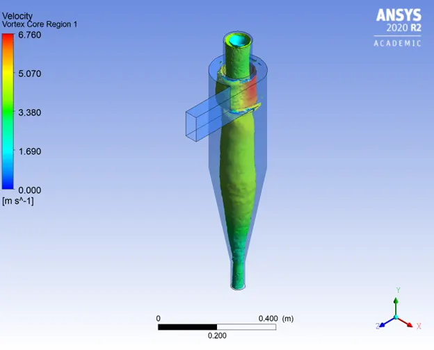
Particle Velocity = 5 m/s