Cyclone Separator Challenge

Aim: To perform an analysis on a cyclone separator model for constant velocity case (3m/s) and a constant particle size (5 μm) case. For the constant velocity case, we must calculate the separation efficiency. For the constant particle case, we must calculate the separation efficiency as well as the pressure drop.

Empirical Models:

1) Iozia and Leith Model: This model is developed based on force balance. Here the particle that is in the vortex experiences the influence of two forces: centrifugal forces and flow resistance. The collection efficiency (nu) of the particle diameter d_pi can be calculated from:

nu = 1/(1+(d_pc/d_pi)^beta)

Here beta is defined as the slope parameter based on statistical analysis.

2) Li and Wang Model: This model includes particle bounce or re-entrainment and turbulent diffusion at the cyclone wall. This model was based on the following assumptions, 1) the radial particle velocity and the radial concentration profile are not constant for uncollected particles within the cyclone. 2) Boundary conditions with the consideration of turbulent diffusion coefficient and particle bounce re-entrainment on the cyclone wall.

3) Koch and Licht Model: This theory recognizes the inherent turbulent nature of cyclones and the distribution of gas residence times within the cyclone. It described particle motion in the entry and collection regions along with the following assumptions: 1) The tangential velocity of a particle is equal to the tangential velocity of the gas flow which means there is no slip. 2) The tangential velocity is related to the radius of cyclone by: `uR^N=const ant`

4) Lapple Model: This model was developed based on force balance without considering the flow resistance. Lapple made an assumption that particle entering the cyclone is evenly distributed across the inlet opening. The particle that travels from the inlet half-width to the wall in the cyclone is collected with 50% efficiency. The semi-empirical relation to calculate a 50% cut diameter,

`d_(pc) = [(9mub)/(2piN_ev_i(rho_p-rho_g))]^(1/2)`

where is the number of revolutions `N_e` and the efficiency of collection of any size of the particle is given by:

`eta_i = 1/(1+(d_(pc)+d_(p i))^2)`

Pre-Processing:

Geometry:

• Open ANSYS> from the analysis system in the toolbox drag Fluid Flow (Fluent) on to the project schematic.
• Right-click on geometry> open Spaceclaim.
• Drag the solid part geometry to the SpaceClaim window. Wait for the geometry to import.
• Go to prepare > enclosed volume > select the three edges > click done.
• Close the space claim window.

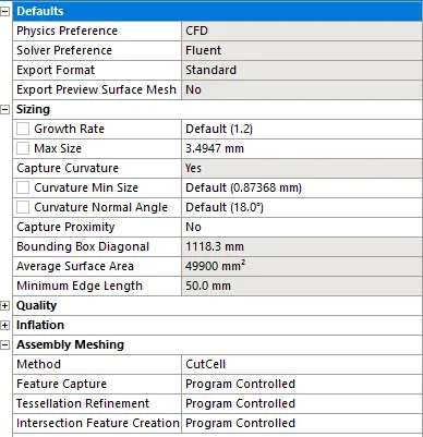
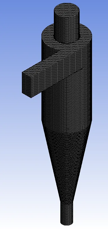
Meshing: Create named selection - inlet, outlet1 and outlet2. Use a mesh size of 3.5mm and in the assembly method use the cut shell method.

Setup:

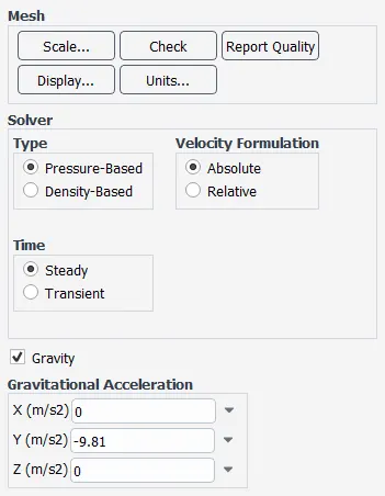
• In general, use a pressure-based solver and turn on gravity in the negative Y direction.

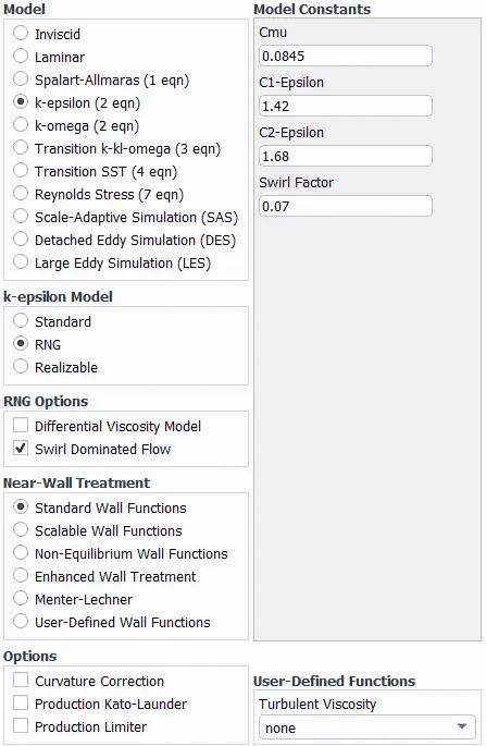
• No moving on to the viscous model, use the k-epsilon model, RNG, and a swirl dominated flow.

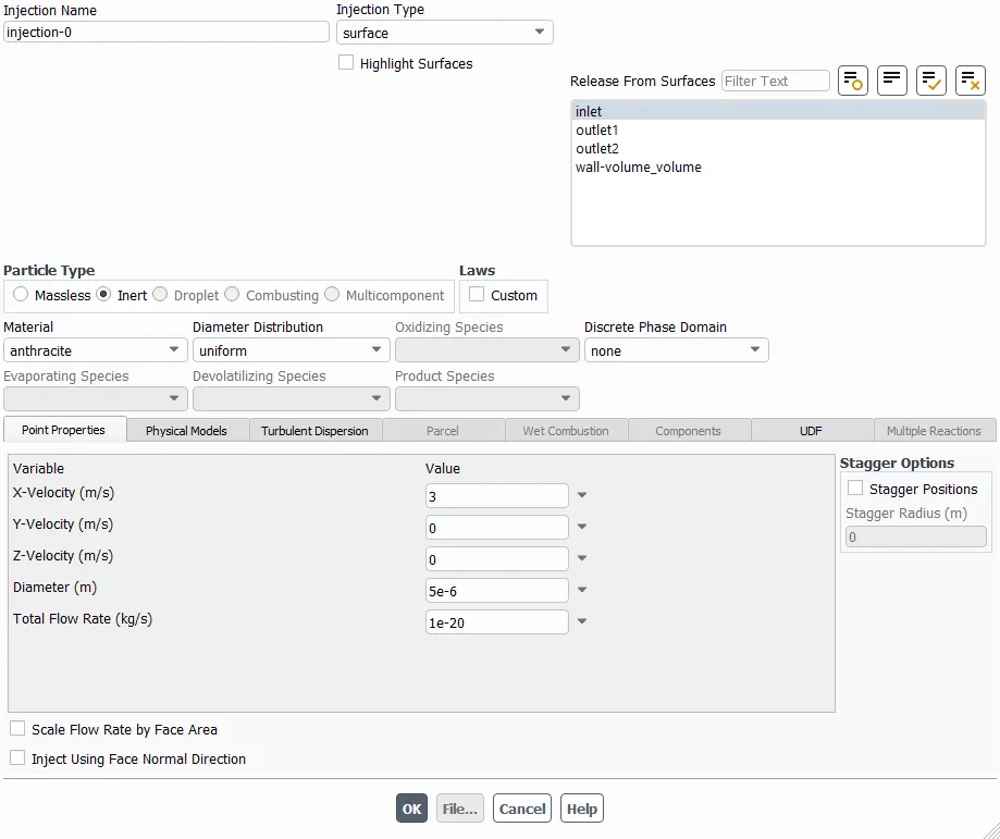
• Also, turn on the discrete phase. Set the particles to inert and add a velocity of the particle in the X-direction by releasing the particles from the inlet surface.

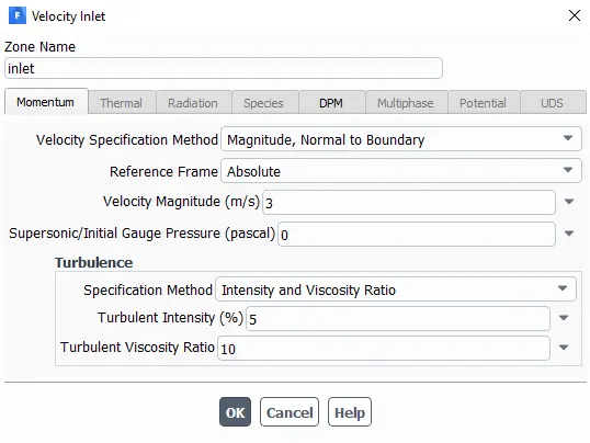
• Moving forward to the boundary conditions, for the DPM at the inlet set it as reflect, the top outlet as an escape, and the bottom outlet as a trap.

• Use standard initialization and run the setup

Results: After the setup has complete simulation, go to file > export > particle history file > and save the file. Record the particles trapped and the particles tracked. Along with this compute the total pressure at the inlet as well as the outlet, to measure the pressure drop.

Post-Processing

Create a streamline plot for the volume. Then import the particle history file and create an animation for the particle history.

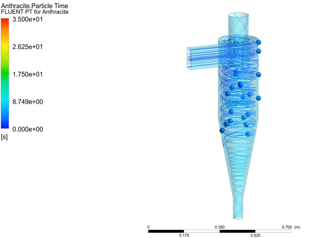
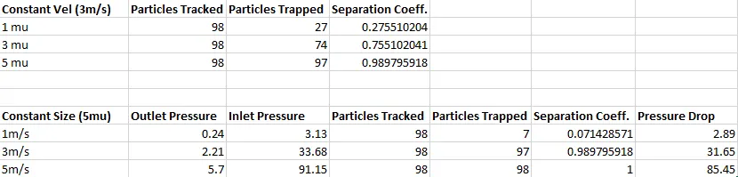
Results: Perform the following steps for the different cases required and obtain the following results.

Separation coeff: Particles tracked/Particles trapped

Pressure Drop: Inlet pressure - Outlet Pressure