Curve Fitting using Python

Objective:

Write a Python Program to curve fit a linear and cubic polynomial for the given Cp data and explain the results.

Curve Fitting:

Curve fitting is the process of constructing a curve, or mathematical function, that has the best fit to a series of data points, possibly subject to constraints. Curve fitting can involve either interpolation, where an exact fit to the data is required, or smoothing, in which a "smooth" function is constructed that approximately fits the data.

Governing Equations:

Linear or first order polynomial: `y = ax+b`

Quadratic or second order polynomial: `y =ax^2 + bx + c`

Cubic or third order polynomial: `y =ax^3 + bx^2 + cx + d`

Curve Fitting for Linear and Cubic Polynomial:

Python Code:

'''
	Curve fit for Linear Polynomial by Giridhar
'''

import math  
import matplotlib.pyplot as plt  
import numpy as np  
from scipy.optimize import curve_fit

# Linear Curve fit Function
def fun(t,a,b,):
	return a*t + b

# Reading Thermodynamics data file
def read_file():
	temperature = []
	cp = []
	for line in open('data','r'):
		values = line.split(',')
		temperature.append(float(values[0]))
		cp.append(float(values[1]))

	return [temperature, cp]	 

# Main program
temperature, cp = read_file()
popt, pcov = curve_fit(fun, temperature, cp)
fit_cp = fun(np.array(temperature),*popt)

plt.plot(temperature, cp,color='blue',linewidth=2.5)
plt.plot(temperature, fit_cp,color='red',linewidth=2.5)
plt.title('Specific heat(cp) Vs Temperature (Linear Polynomial)')
plt.legend(['Actual data','Curve fit'])
plt.xlabel('Temperature[K]')
plt.ylabel('Specific heat(cp)')
plt.grid()
plt.savefig('case_1')
plt.show()


'''
	Curve fit for Cubic Polynomial by Giridhar
'''

# Cubic Curve fit Function
def fun(t,a,b,c,d):
	return a*pow(t,3) + b*pow(t,2) + c*t + d

# Reading Thermodynamics data file
def read_file():
	temperature = []
	cp = []
	for line in open('data','r'):
		values = line.split(',')
		temperature.append(float(values[0]))
		cp.append(float(values[1]))

	return [temperature, cp]	 


# Main program
temperature, cp = read_file()
popt, pcov = curve_fit(fun, temperature, cp)
fit_cp = fun(np.array(temperature),*popt)

plt.plot(temperature, cp,color='blue',linewidth=2.5)
plt.plot(temperature, fit_cp,color='red',linewidth=2.5)
plt.title('Specific heat(cp) Vs Temperature (Cubic Polynomial)')
plt.legend(['Actual data','Curve fit'])
plt.xlabel('Temperature[K]')
plt.ylabel('Specific heat(cp)')
plt.grid()
plt.savefig('case_2')
plt.show()

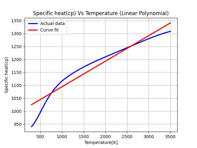
Specific heat(cp) Vs Temperature (Linear Polynomial):

Specific heat(cp) Vs Temperature (Cubic Polynomial):

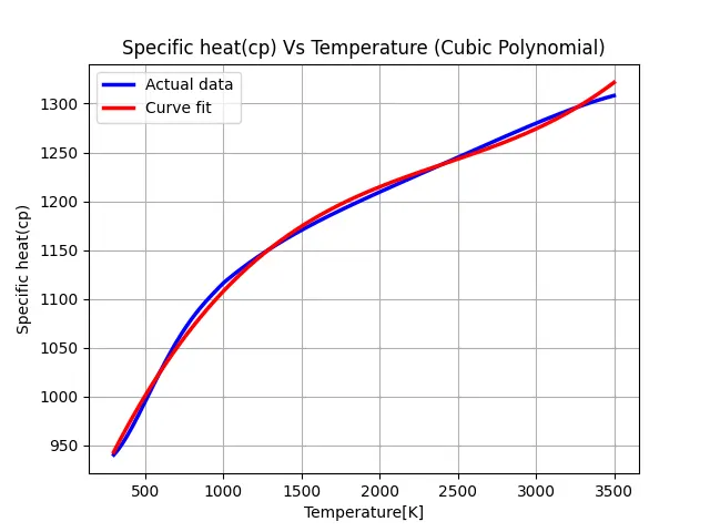
With an increase in order of Polynomial, the curve fit gets better.

Python Code Explanation:

• Required modules are imported.
• A function is created for both linear and cubic polynomial seperately.
• Another function is created to read the provided Thermodynamics file.
• Required commands are provided for curve fitting the T and cp according to polynomial.
• Required commands to plot and save the plot are provided.

What does popt and pcov mean?

popt and pocv are the outputs of the function curve_fit. popt is the array that contains the optimal parameters or the optimum values of the coefficients of the cubic equation. pcov is a 2D array that contains the estimated covariance of the parameters in popt.

What does np.array(temperature) do?

It generates an array and stores the different values of the temperature and passes the generated value to the NumPy for numerical calculation in python.

What does the * in *popt mean?

*popt is used to expand the list of values stored in the array 'popt' into the arguments of the function.

Write code to fit a linear and cubic polynomial for the Cp data. Explain if your results are good or bad.

The results for the linear polynomial is not good as the actual data does not obey the linear equation.

The results for the Cubic polynomial is good but not perfect as both the actual plot and the curve fit plot flows the same plot.

What needs to be done in order to make the curve fit perfect?