CURVE FITTING FOR THE GIVEN THERMAL DATA USING PYTHON

OBJECTIVE:

The primary objective of the project is to find a function that illustrates the given thermal data accurately. This is done with the help of curve fitting method using Python.

PROBLEM STATEMENT:

Given is a file of thermal data containing the temperature of oxygen and the corresponding specific heat capacity. It needs to be read and imported and a suitable function is defined to illustrate the data.

PROCEDURE:

As the first step, the essential libraries are imported first. The next step of the project is to read the given file using an user defined function. The temperaure and specific heat capacities values are separted by commas and then they are appended into separated arrays.

Then the Optimal parameters(popt) and Covariance(pcov) are calculated by the inbuilt function called curve_fit from scipy.optimize module.

popt:

popt means the optimal parameters, that is, the optimal coefficients of the defined equation in which the sum of the squared residulas are minimized.

For example in a quadratic equation,

`ax^2 + bx + c = 0`

a,b,c are the popt values(which are optimal)

pcov:

pcov is the covariance of the popt. This means the joint variability of the popt values.If the greater values of one variable mainly correspond with the greater values of the other variable, and the same holds for the lesser values, the covariance is positive.

In the opposite case, when the greater values of one variable mainly correspond to the lesser values of the other, the covariance is negative.The sign of the covariance therefore shows the tendency in the linear relationship between the variables.

Then the fitting 'cp' that is, the optimal specific heat capacity(fit_cp) is calculated by passing the temperature values and the calculated popt values to the user defined function.

Need for np.array(temperature):

Here the temperature values are passed as a 1D array to the user defined function which defines the data. As it is an array, for each value of temperature, the corresponding value of specific heat is calculated.

Significance of '*' in '*popt':

The '*' operator is used to pass all the values of the calculated optimal coefficients which is 'popt' to the u.d.f. It contains the parameters "a,b,c,d".

Program snippet for cubic polynomial and linear function:

The following program shows the curve fitting using a cubic polynomial function and a linear function.

# CURVE FITTING

# Importing essential libraries
import matplotlib.pyplot as plt
import numpy as np
from scipy.optimize import curve_fit

# User defined polynomial function for curve fitting
def func(t,a,b,c,d):
	return a*pow(t,3) + b*pow(t,2) + c*t + d

# User defined linear function for curve fitting
def func2(t,a,b):
	return a*t + b

# User defined function to read the thermodynamic data file
def read_file():
	temperature = []
	cp = []

	# Loop to read each line and import data
	for line in open('data','r'):
		values = line.split(',')
		temperature.append(float(values[0]))
		cp.append(float(values[1]))

	return [temperature, cp]

# Main program
temperature, cp = read_file()

# Calculating optimal coefficients and covariance b/w temperature and cp
popt, pcov = curve_fit(func, temperature, cp)

# Caculating the new cp which form a curve that fits
fit_cp = func(np.array(temperature), *popt)

# Calculating optimal coefficients and covariance b/w temperature and cp for linear function 
popt2, pcov2 = curve_fit(func2, temperature, cp)

# Caculating the new cp for the linear function
fit_cp2 = func2(np.array(temperature), *popt2)


# Finding the "Sum of Squares due to Error" to find the best fit
error_poly = 0

for i in range(3199):
	error_poly = pow((cp[i] - func(temperature[i], *popt)),2)

	error_poly += error_poly

error_line = 0

for i in range(3199):
	error_line = pow((cp[i] - func2(temperature[i], *popt2)),2)

	error_line += error_line

# Printing the SSE's
print("SSE of Cubic Polynomial function = ",error_poly)
print("SSE of Linear function = ",error_line)

# Plotting the data
plt.plot(temperature,cp,'b-')
plt.plot(temperature,fit_cp,'r-')
plt.plot(temperature,fit_cp2,'g-')
plt.legend(['Actual data', 'Cubic Polynomial', 'Linear function'])
plt.title('CURVE FITTING FOR THERMAL DATA')
plt.xlabel('Temperature')
plt.ylabel('Specific heat capacity')
plt.show()

Output:

Plot:

INFERENCE:

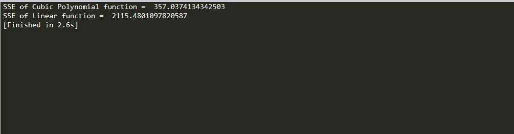
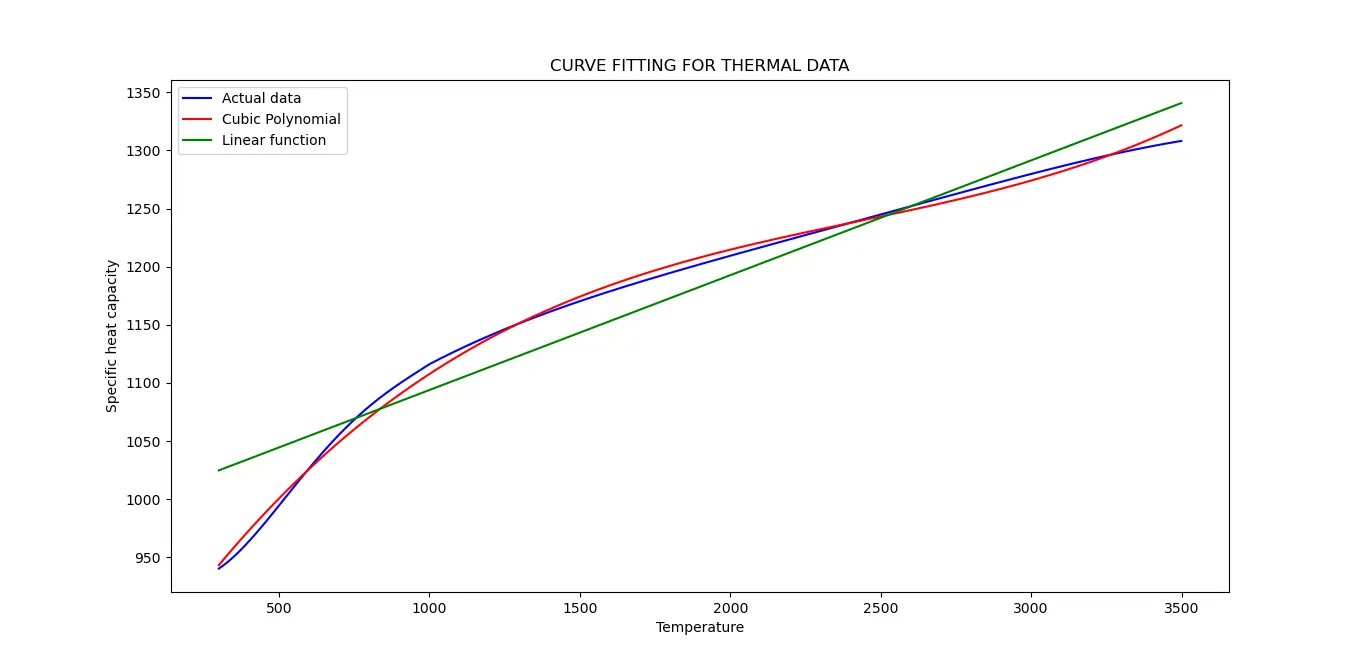
In the output, the "Sum of the squares due to error(SSE)" values are calculated and printed for each function. It is the measure of the quality of the fit. Lesser the SSE, better the fit. So from the values, it is evident that the cubic polynomial function is about 6 times fitter than the linear function.

From the plots also, it shows that the SSE values are correct in a graphical manner. As we can see, the cubic polynomial mimics the original data in a near perfect manner. But the linear function is far from being a good fit.

Quintic polynomial function:

Eventhough the cubic polynomial function is a sort of good fit, but it can be better. So a Quintic polynomial function is used to define the curve. The program snippet is as follow.

Program snippet for Quintic function:

# CURVE FITTING WITH QUINTIC POLYNOMIAL

# Importing essential libraries
import matplotlib.pyplot as plt
import numpy as np
from scipy.optimize import curve_fit

# User defined polynomial function for curve fitting
def func(t,a,b,c,d,e,f):
	return a*pow(t,5) + b*pow(t,4) + c*pow(t,3) + d*pow(t,2) + e*t + f 

# User defined function to read the thermodynamic data file
def read_file():
	temperature = []
	cp = []

	# Loop to read each line and import data
	for line in open('data','r'):
		values = line.split(',')
		temperature.append(float(values[0]))
		cp.append(float(values[1]))

	return [temperature, cp]

# Main program
temperature, cp = read_file()

# Calculating optimal coefficients and covariance b/w temperature and cp
popt, pcov = curve_fit(func, temperature, cp)

# Caculating the new cp which form a curve that fits
fit_cp = func(np.array(temperature), *popt)

# Finding the "Sum of Squares due to Error" to find the best fit
error_poly = 0

for i in range(3199):
	error_poly = pow((cp[i] - func(temperature[i], *popt)),2)

	error_poly += error_poly

# Printing the SSE's
print("SSE of Quintic Polynomial function = ",error_poly)

# Plotting the data
plt.plot(temperature,cp,'b-')
plt.plot(temperature,fit_cp,'r-')
plt.legend(['Actual data', 'Quintic Polynomial'])
plt.title('CURVE FITTING FOR THERMAL DATA')
plt.xlabel('Temperature')
plt.ylabel('Specific heat capacity')
plt.show()

Output:

Plot:

INFERENCE:

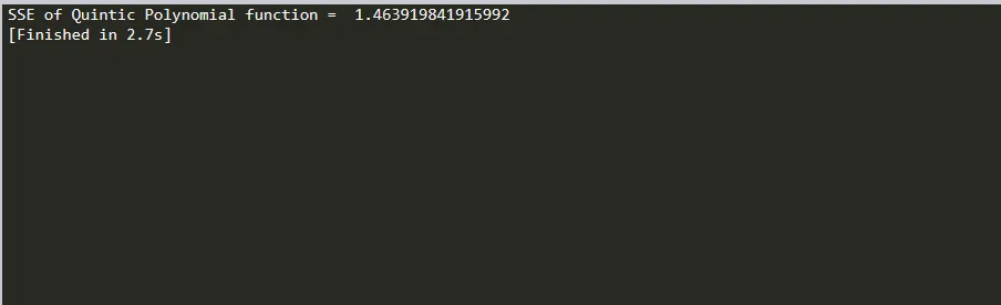
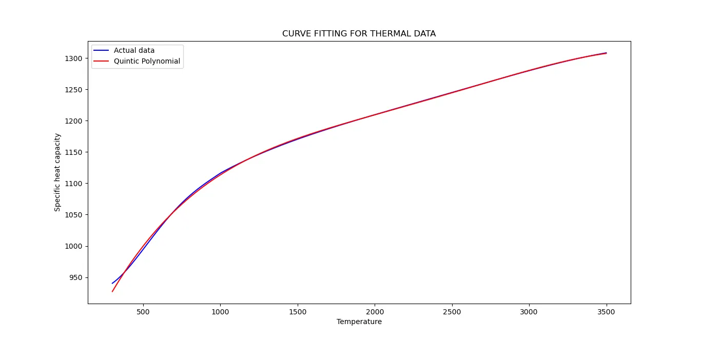
The SSE of the quintic polynomial is calculated as 1.463 which is almost 300 times better than that of the cubic polynomial which has a SSE of 357.03. In the plot also, it is evident that the quintic polynomial curve is in great fit with the original data.

CONCLUSION:

These results can be interpreted as, that the polynomial function is better in describing the given thermal data than the linear function. Also, the quality of the fit drastically increases when the degrees of the polynomial are increases. This is because, as the degree of the polynomial increases, the number of roots are also increases. This makes the curve well defined and will have a better fit.