Curve Fitting

AIM:

Fit a polynomial curve to approximate the given dataset.

Description:

Curve Fitting is a technique used to model discrete data. In this method, a curve is selected so that it the total error for approximation is least or minimum. To do this a curve of unknown coefficients is assumed to model the data. Then the sum of squares of error at each point of the curve is calculated. This Error is minimized to find the Unknowns coefficients.

Let, [x(i), y(i)] be the given data set. Where, 0<=i<=N.

A(i)=A₁(x(i)) ⁿ +A₂(x(i)) ^n-1 +.........................................................+A_n(x(i))⁰

Error=_i∑(y(i)-A(i))²

Differentiating Error with respect to various coefficients {A1, A2, .........., An} and equating it to zero gives the unknown variables their values.

Method^:

1. The data is loaded into a matrix.
2. The total data is made into separate vectors.
3. Now using the 'polyfit' command the data is fitted into a polynomial of the order specified.
4. After finding the unknown coefficients the data values at each x(i) are predicted and stored as separate Vector.
5. Now, if required both original and predicted data is plotted for comparison.

Code:

%Setting up a fresh workspace
clear all;
close all;
clc;

%Reading the data
cp_data=load('data');

%organizing into variables
temp=cp_data(:,1);
cp_values=cp_data(:,2);

for i=0:10
coeff=polyfit(temp,cp_values,i);%fitting multiple curves
predictedcp=polyval(coeff,temp);%caluclating the prdicted values
%comparing the oroginal data with predicted one
grid on;
plot(temp,predictedcp,'linewidth',3,temp,cp_values,'linewidth',3);
xlabel("Temparature");
ylabel("Cp");
%creating an animation
title(['fontsize{30}order:' num2str(i)]);
pause(0.3);
text=sprintf('output%d.png',i);
saveas (gca,text);
endfor
for i=0:10
coeff=polyfit(temp,cp_values,i);%fitting multiple curves
predictedcp=polyval(coeff,temp);%caluclating the prdicted values
%Error Estimation
if(i!=0)
Error(i)=0;
for j=1:length(temp)%finding error for diffrent order of curve fitting
Error(i)= Error(i)+(cp_values(j)-predictedcp(j))^2;
endfor
end
endfor
p=1:10;
figure(2);
grid on;
plot(p,Error,'linewidth',3,'marker','o');%plotting error vs order of approximation
xlabel("Order");
ylabel("Error");

Result:

Here, the data is approximated with polynomials of different orders from 1 to 10 and they are compared. After examining the results, it is found that the degree of goodness of fit improves with order. But, for order greater than 4 the improvement is very minimal. So, the polynomial of degree 4 can be considered as best fit. Even the 3rd order also seems to be reasonably good.

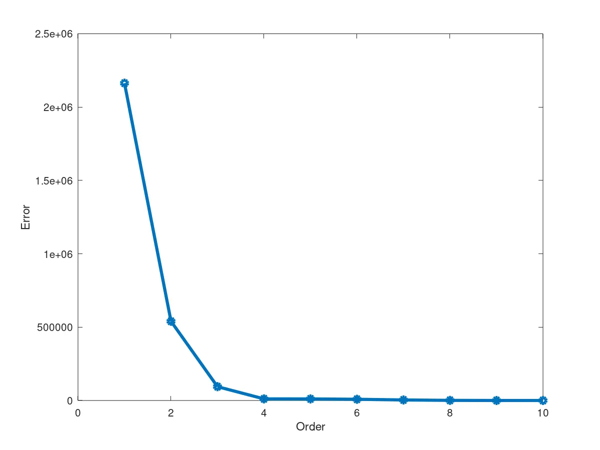
Modelling Approximations :