Conjugate Heat Transfer Analysis on a graphics card.

Objective: In this challenge, we will be conducting a conjugate heat transfer analysis on a model of a graphics card with three different inlet velocities between 1m/s to 5m/s of air at 300K and a heat source at the processor. A conjugate heat transfer analysis is used when the fluids and solids involved in the simulations undergo a variation in temperature due to the thermal interactions between them at the interfaces. This type of analysis can be used in the simulation of heat exchangers, analysis in cooling of electronic equipment, and general heating and cooling system.

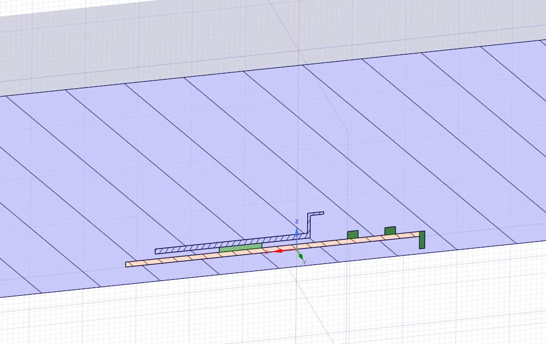
Solving and modeling approach: The provided model file is imported in space-claim. An enclosure is created using the graphics card model. Then we ensure that the analysis is set to share topology so that the mesh formed are connected between the volume and the solid part. A fine tetra mesh is created both in the fluid volume and solid volume. As we are going to analyze the wall HTC we use an element of smaller size for the solid volume. We also add an inflation layer using the first layer method at the fluid-solid interface. This is done to apply the appropriate wall yplus or wall shear in the simulation. Then we move forward with setup, where we use a pressure-based formulation in a steady-state analysis. In the model, we set energy on and used the k-epsilon viscous method. For the materials, we use silicon for the transistors, processor and the capacitor in the model, the other parts used are aluminum and the electric board is of copper with air as the fluid. Here, we use a velocity inlet at 300K and pressure outlet as boundary conditions. After the simulation is run for around 1500 iterations we obtain the heat transfer coefficient at the interface.

Pre-processing

Geometry:

• Open ANSYS> from the analysis system in the toolbox drag Fluid Flow (Fluent) on to the project schematic.
• Right-click on geometry> open Spaceclaim.
• Drag the solid part geometry to the SpaceClaim window. Wait for the geometry to import.
• In the main design,> change share topology to share.
• Click on workbench > click share > select the body.
• Ensure that there are no duplicates or interference.
• Close the space claim window.

Mesh:

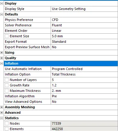
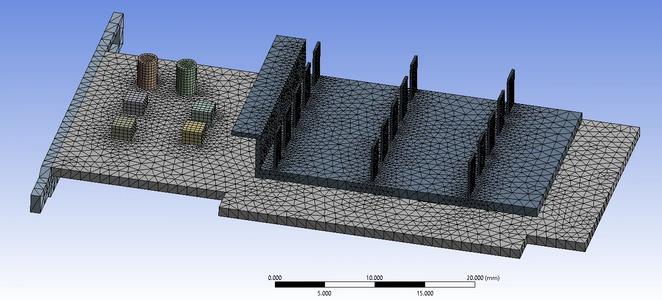
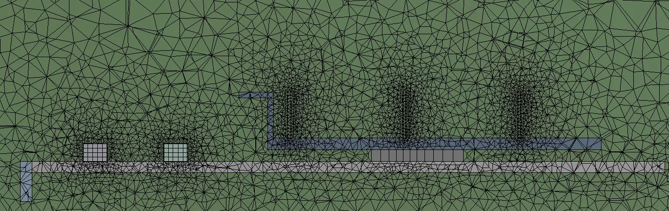
Here i have added edge sizing to the fin edges and the transistors. This was done to produce a finer mesh in the fins and to obtain an appropriate hexa mesh in the capacitor since there are cubic shaped. Then body sizing was added to the fins structure and the graphic card base. This produces the following mesh.

Setup:

• We start with mesh check. In domain > go to mesh > select check > Wait for mesh checking results.
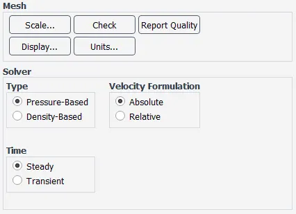
• In general, we will be using a pressure-based model with absolute velocity formulation for steady-state analysis.
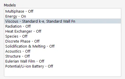
• Go to models > turn on energy > in the viscous model: set it as K-epsilon.

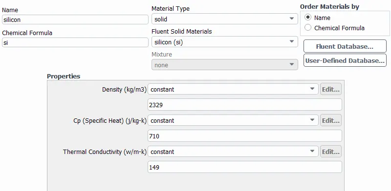
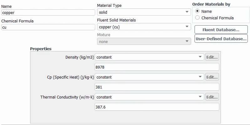
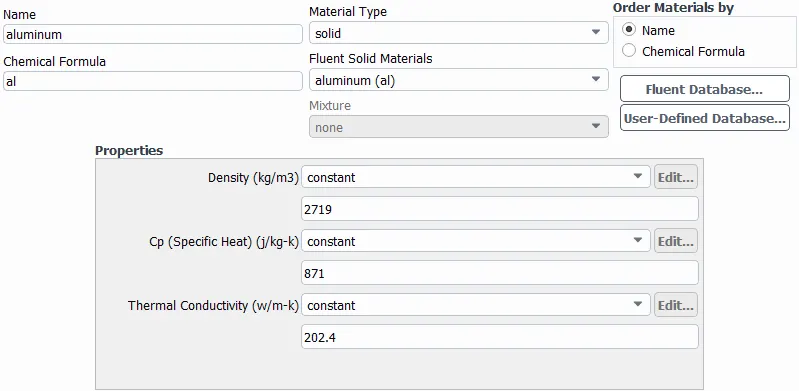
• In materials the fluid material is air and the solid material is aluminum, silicon and copper. The semiconductors and the processor is made of silicon, the base is copper ,and fins are aluminium.
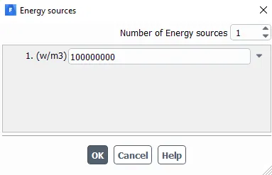
• We go to the cell zone conditions and change the type for the model as solid and assign the materials as metioned above. In the processor, select on source terms and add an energy source.

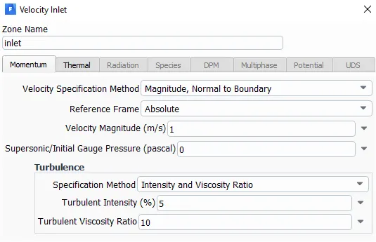
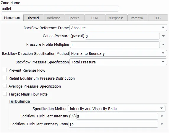
• Now we move on to the boundary conditions. For inlet it will be a velocity inlet, the outlet will be pressure outlet.
• For the inlet, we set the inlet velocity as 1m/s, 3m/s and 5m/s respectively, and set the temperature at 300 K.

Solution:

• Now we move to initialization and initialize using a hybrid method.
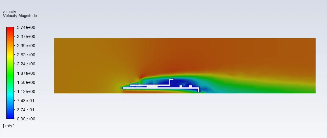
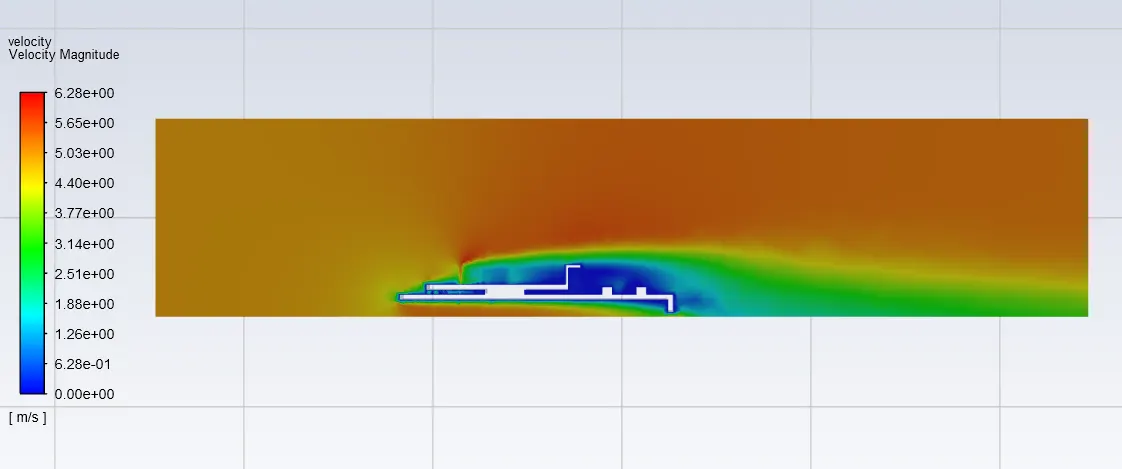
• We go to results > graphics > contours > new > crate a temperature contour at the surface of the graphic card model. Similarly we create a velocity contour for a mid section plane.
• In solutions > go to activities > create > select scene animation > then select the temperature contour as the entity.
• Run the calculation for 1500 iterations.

Post Processor:After the setup simulation is completed we double click results. The results to be obtained are:

1. Velocity contours at cross-sections.
2. Temperature contours for the three different velocities.
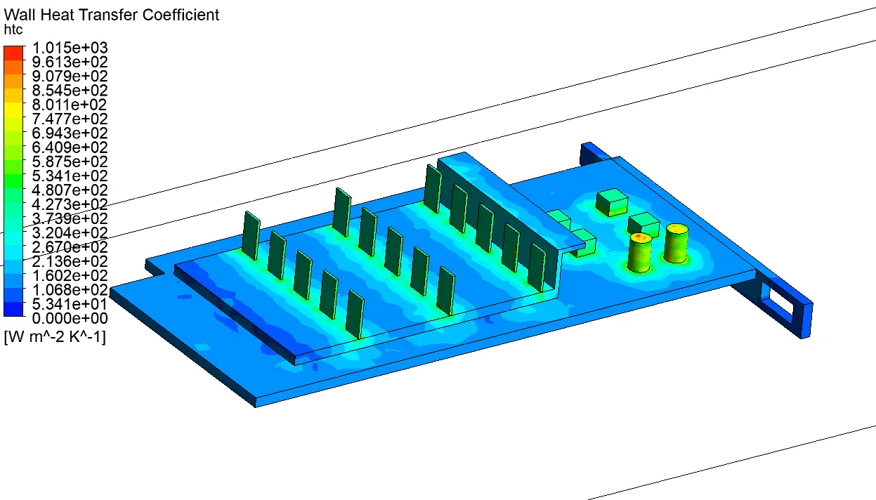
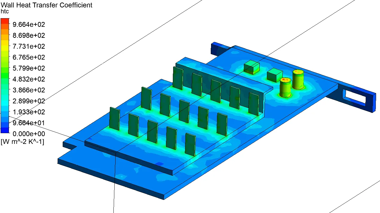
3. Wall Heat Transfer Coefficient contour.

For 1m/s

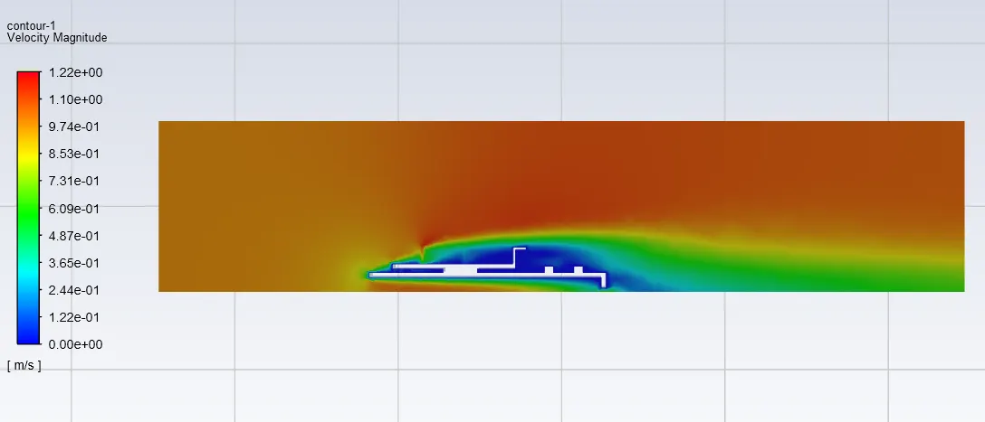
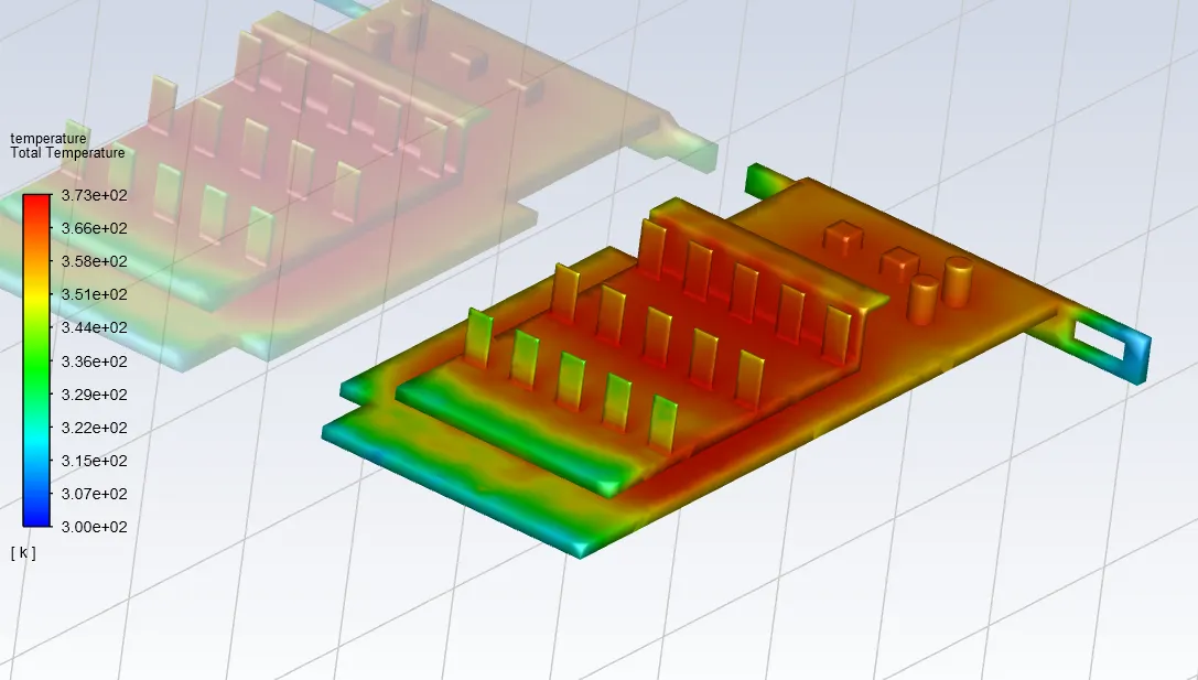
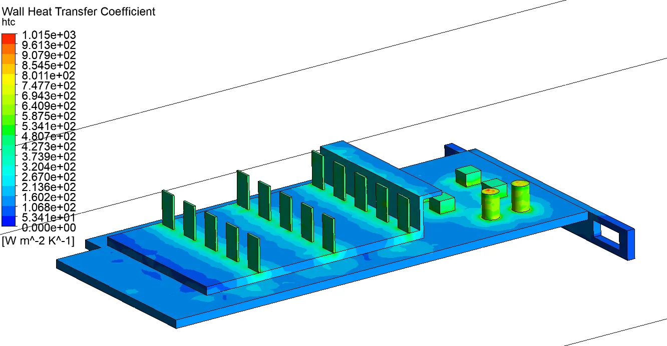
Maximum Temperature Obtained is 372.85K

Maximum Heat transfer Coefficient 1014.71K

For 3m/s

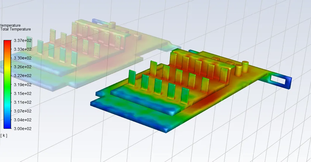
Maximum Temperature Obtained is 337.01K

Maximum Heat transfer Coefficient 1014.71K

For 5m/s

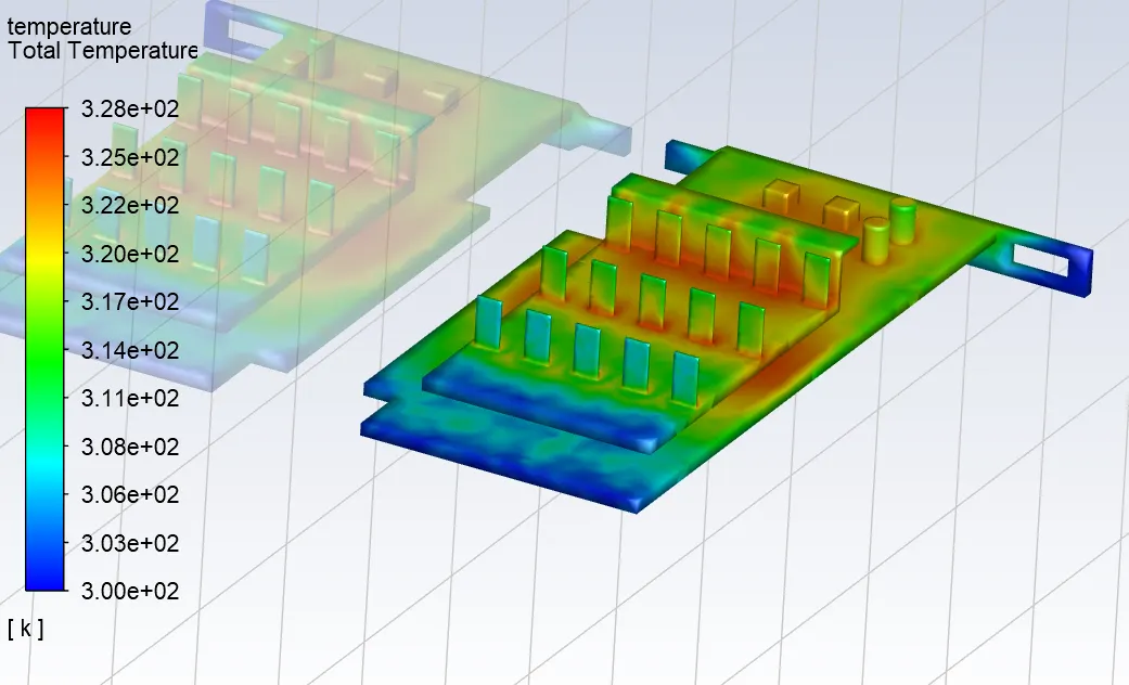
Maximum Temperature Obtained is 328K

Maximum Heat transfer Coefficient 1014.71 w/m2K

Processor Results:

For 1m/s

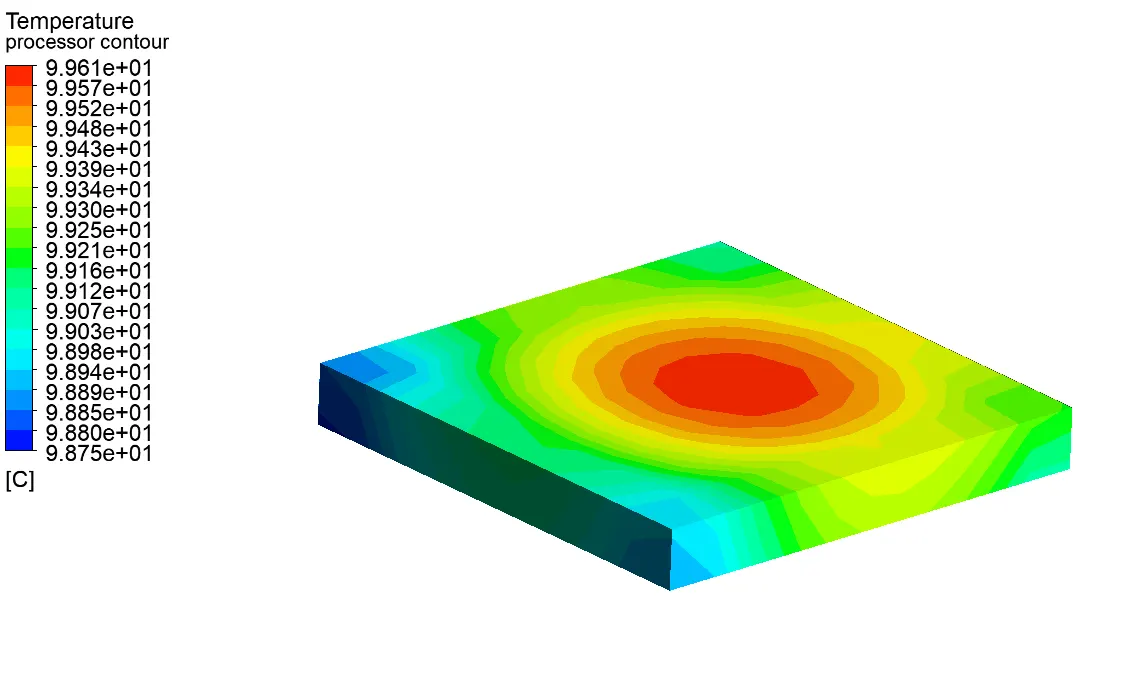
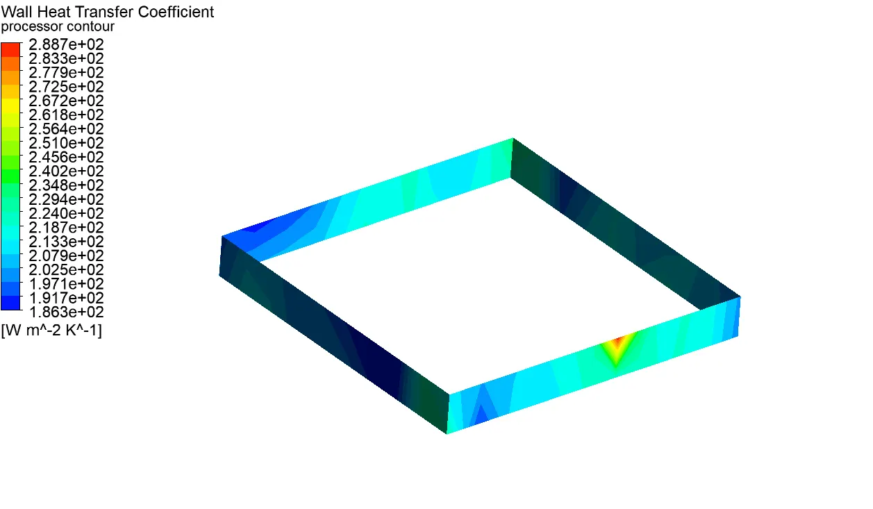
Maximum Temperature Obtained is 99.611C

Maximum Heat transfer Coefficient 288.712 w/m2K

For 3m/s

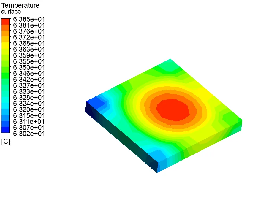
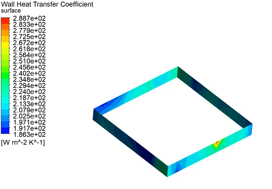
Maximum Temperature Obtained is 63.49C

Maximum Heat transfer Coefficient 288.712 w/m2K

For 5m/s

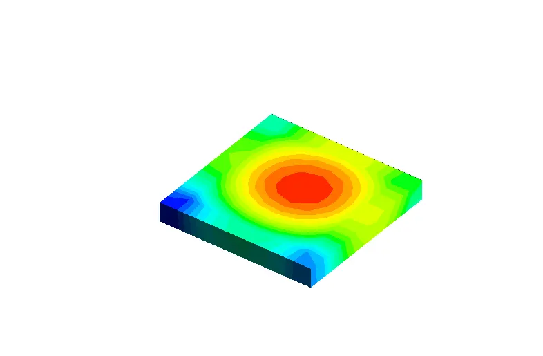
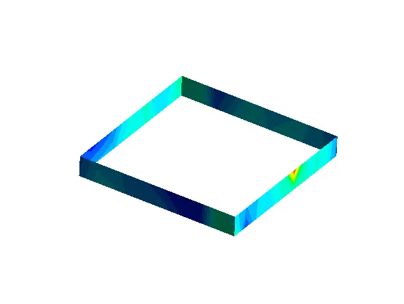
Maximum Temperature Obtained is 54.8C

Maximum Heat transfer Coefficient 288.712 w/m2K

Result

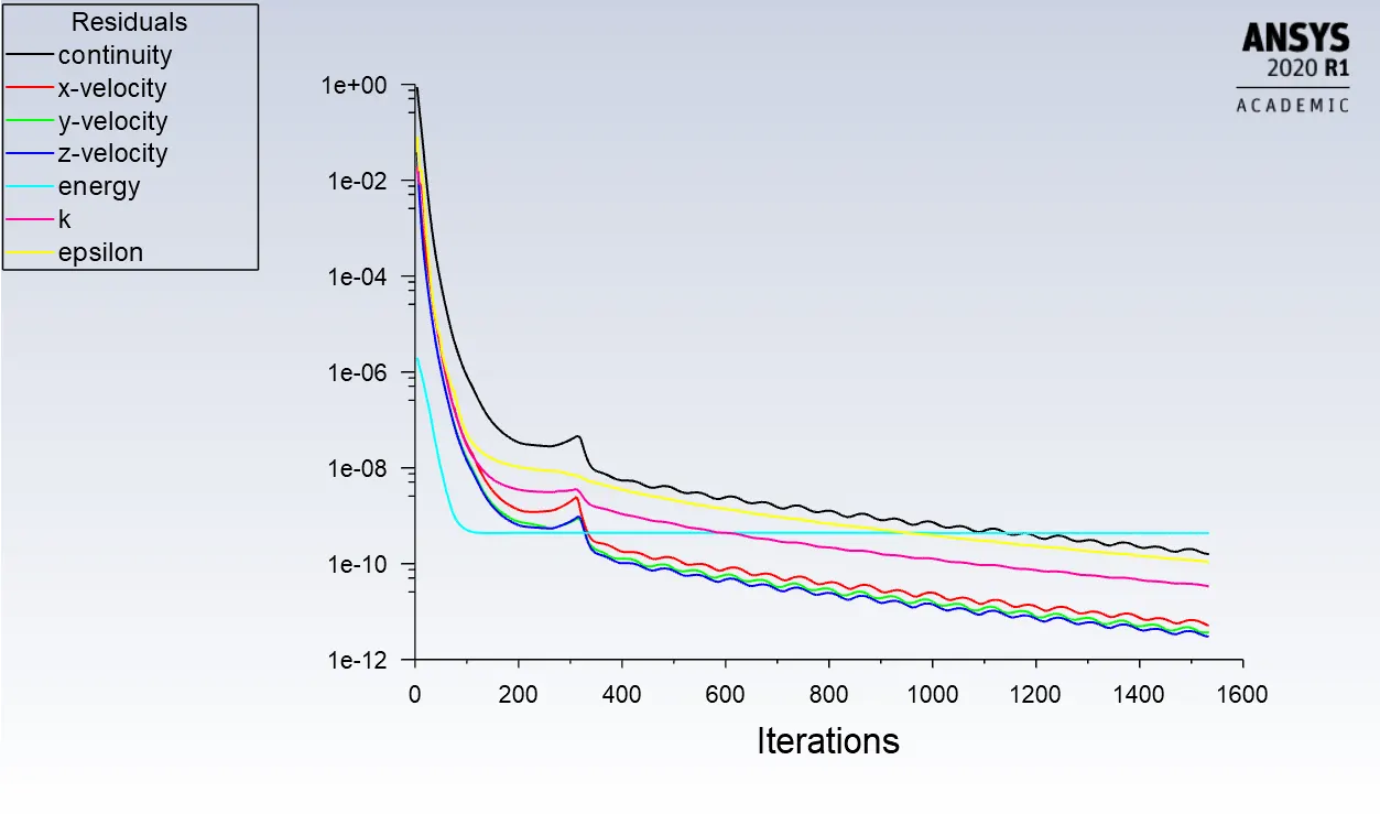
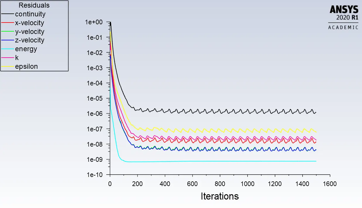
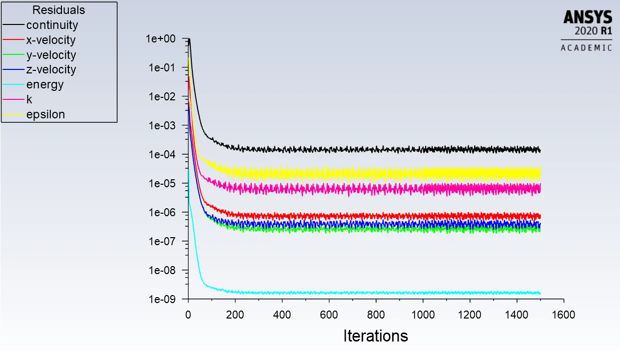
The conjugate heat transfer analysis was successfully conducted on the given graphics card model. The maximum temperature drop was obtained with air speed of 5m/s which is 54.8C and is great when compared to the inlet velocity of 1m/s. Also the residual plots show that the simulations have converged and this can also be seen in the animation files. Heat transfer coefficient for all the cases stay the same as they are area and temperature dependent.