Combined Slip Correction Model using Pacejka Magic Formula

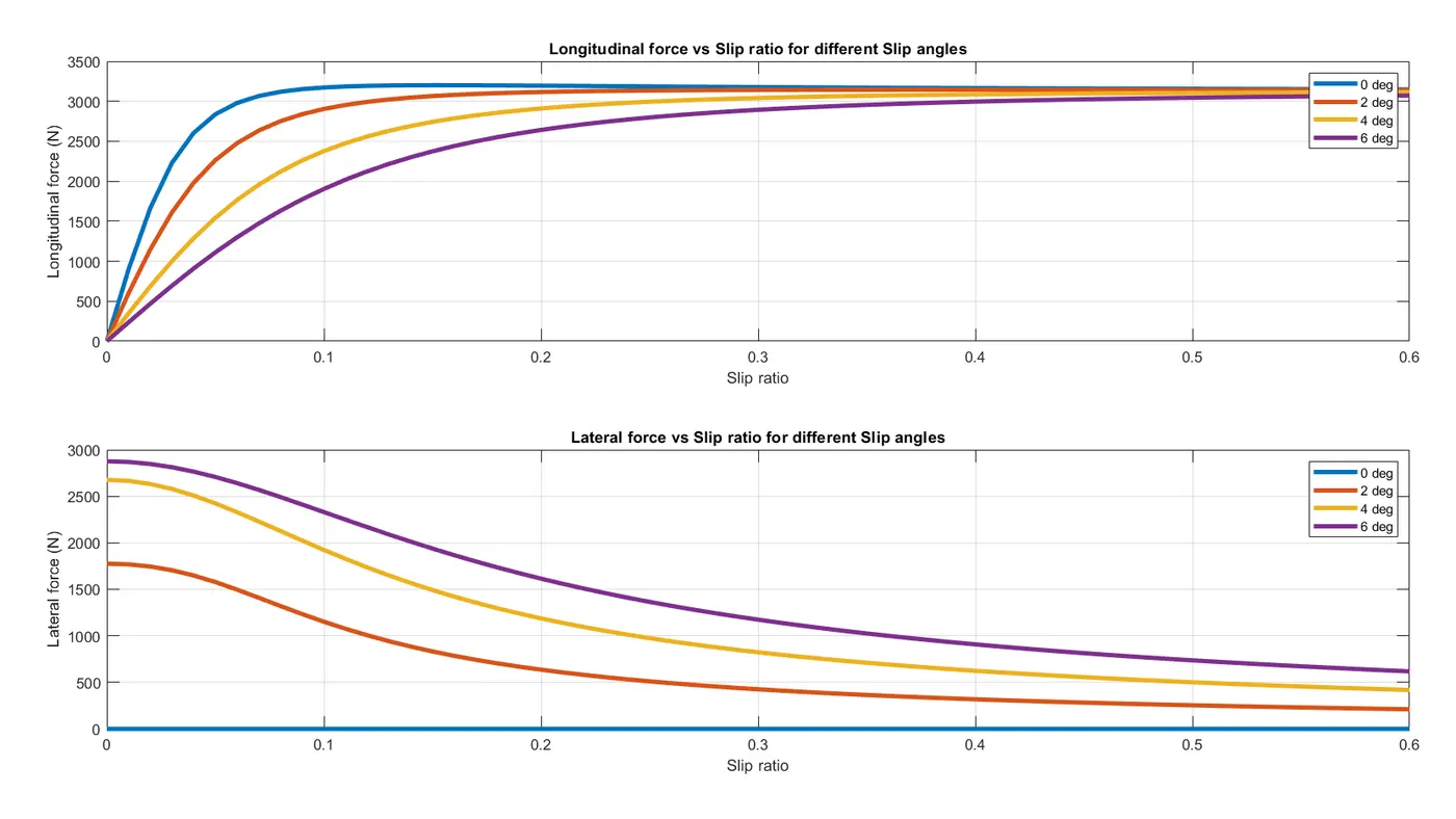
AIM: To show the effect of different slip angles on longitudinal force and lateral force vs slip ratio relationship; and different slip ratios on longitudinal force and lateral force vs slip angle relationship.

GIVEN DATA:

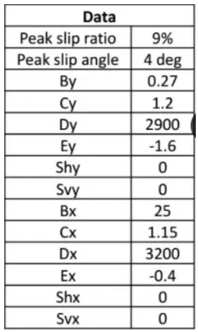
OBJECTIVE: To plot the longitudinal force vs lateral force relationship using:

- Slip angles (0 deg, 2 deg, 4 deg and 6 deg) influence the force (Fx and Fy) vs slip ratio relationship (sweep from 0 to 60%)

- Slip ratios (0%, 3%, 6% and 9%) influence the force (Fx and Fy) vs slip angle relationship (sweep from 0 to 20 deg)

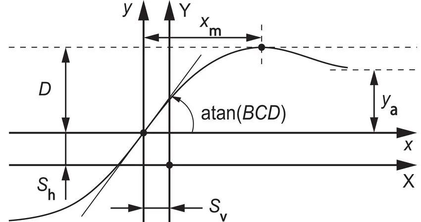
GOVERNING EQUATION: The Packejka Magic Formula can be given as:

`Y(X) = D.sin[C.tan^(_1){Bx - E(Bx - tan^(-1)(Bx))}]` `Y(X) = y(x) + S_v` `x = X + S_h` where; `Y(X)` = Cornering force, Braking force or Self-aligning moment `x` = Slip angle or Skid ratio `B` = Stiffness factor `C` = Shape factor (controls stretching in X-directon) `C` = 1.3 ... (Lateral force) `C` = 1.65 ... (Longitudinal force) `C` = 2.4 ... (Self-aligning moment) `D` = Peak value or Peak factor `E` = Curvature factor (affects transition between and position X_m at which peak value occurs) `E = frac(Bx_m - tan(frac(pi)(2C)))(Bx_m - tan^(-1)(Bx_m)` `S_v` , `S_h` = Vertical shift and Horizontal shift (offsets to account for camber thrust, conicity, ply steer or rolling resistance)

SOLUTION:

Programming Language: MATLAB

Code #1:

% Effect of Slip angles on Force (Longitudinal and Lateral) vs Slip ratio relationship

% Input data:

s_xp = 0.09;   % Peak slip ratio
alpha_p = 4;   % Peak slip angle

% Pac Coefficients
By = 0.27; Cy = 1.2; Dy = 2900; Ey = -1.6; Shy = 0; Svy = 0;   % Lateral direction
Bx = 25; Cx = 1.15; Dx = 3200; Ex = -0.4; Shx = 0; Svx = 0;    % Longitudinal direction


% Solution:

for i=1:4   % Slip angle loop
    alpha = (i-1)*2 + 0.0001;   % (0 deg,2 deg,4 deg,6 deg)
    
    for j=1:61   % Slip ratio loop
        s(j) = (j-1)*0.01;   % (0 to 60 %)
        s_x = s(j);
        
        % Normalized slip factors
        s_x_star = s_x/s_xp;
        alpha_star = alpha/alpha_p;
        
        % Resultant slip
        s_star = ((s_x_star)^2 + (alpha_star)^2)^0.5;
        
        % Modified slip factors
        s_x_mod = s_star*s_xp;
        alpha_mod = s_star*alpha_p;
        
        % Longitudinal force calculations
        s_x_final = s_x_mod + Shx;   % Including horizontal shift
        f_x(i,j) = (s_x_star/s_star)*Dx*sin(Cx*atan(Bx*s_x_final - Ex*(Bx*s_x_final - atan(Bx*s_x_final))));
        F_x(i,j) = f_x(i,j) + Svx;   % Including vertical shift

        % Lateral force calculations
        alpha_final = alpha_mod + Shy;   % Including horizontal shift
        f_y(i,j) = (alpha_star/s_star)*Dy*sin(Cy*atan(By*alpha_final - Ey*(By*alpha_final - atan(By*alpha_final))));
        F_y(i,j) = f_y(i,j) + Svy;   % Including vertical shift
        
    end
end


% Plot:
   
subplot(2,1,1)
plot(s,F_x,'linewidth',3)
xlabel('Slip ratio')
ylabel('Longitudinal force (N)')
title('Longitudinal force vs Slip ratio for different Slip angles')
legend('0 deg','2 deg','4 deg','6 deg')
grid on
hold on

subplot(2,1,2)
plot(s,F_y,'linewidth',3)
xlabel('Slip ratio')
ylabel('Lateral force (N)')
title('Lateral force vs Slip ratio for different Slip angles')
legend('0 deg','2 deg','4 deg','6 deg')
grid on

Code #2:

% Effect of Slip ratios on Force (Longitudinal and Lateral) vs Slip angle relationship

% Input data:

s_xp = 0.09;   % Peak slip ratio
alpha_p = 4;   % Peak slip angle

% Pac Coefficients
By = 0.27; Cy = 1.2; Dy = 2900; Ey = -1.6; Shy = 0; Svy = 0;   % Lateral direction
Bx = 25; Cx = 1.15; Dx = 3200; Ex = -0.4; Shx = 0; Svx = 0;    % Longitudinal direction


% Solution:

for i=1:4   % Slip ratio loop
    s_x = (i-1)*0.03;   % (0 %,3 %,6 %,9 %)
    
    for j=1:21   % Slip angle loop
        alpha1(j) = (j-1) + 0.00001;   % (0 to 20 deg)
        alpha = alpha1(j);
        
        % Normalized slip factors
        s_x_star = s_x/s_xp;
        alpha_star = alpha/alpha_p;
        
        % Resultant slip
        s_star = ((s_x_star)^2 + (alpha_star)^2)^0.5;
        
        % Modified slip factors
        s_x_mod = s_star*s_xp;
        alpha_mod = s_star*alpha_p;
        
        % Longitudinal force calculations
        s_x_final = s_x_mod + Shx;   % Including horizontal shift
        f_x(i,j) = (s_x_star/s_star)*Dx*sin(Cx*atan(Bx*s_x_final - Ex*(Bx*s_x_final - atan(Bx*s_x_final))));
        F_x(i,j) = f_x(i,j) + Svx;   % Including vertical shift

        % Lateral force calculations
        alpha_final = alpha_mod + Shy;   % Including horizontal shift
        f_y(i,j) = (alpha_star/s_star)*Dy*sin(Cy*atan(By*alpha_final - Ey*(By*alpha_final - atan(By*alpha_final))));
        F_y(i,j) = f_y(i,j) + Svy;   % Including vertical shift
        
    end
end


% Plot:
   
subplot(2,1,1)
plot(alpha1,F_x,'linewidth',3)
xlabel('Slip angle')
ylabel('Longitudinal force (N)')
title('Longitudinal force vs Slip angle for different Slip ratios')
legend('0 %','3 %','6 %','9 %')
grid on
hold on

subplot(2,1,2)
plot(alpha1,F_y,'linewidth',3)
xlabel('Slip angle')
ylabel('Lateral force (N)')
title('Lateral force vs Slip angle for different Slip ratios')
legend('0 %','3 %','6 %','9 %')
grid on

Output #1:

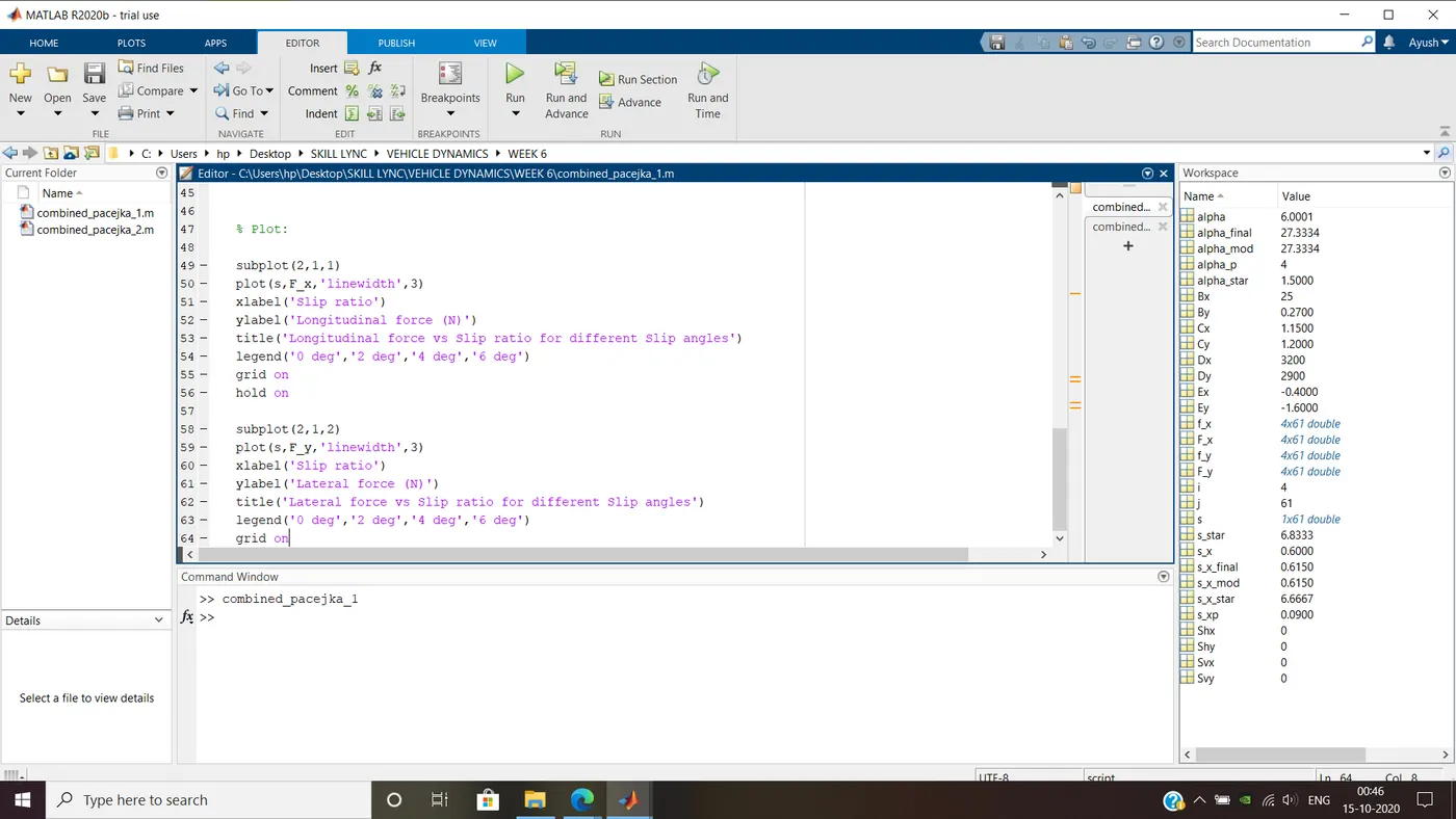
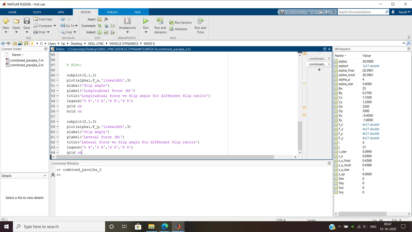
Output #2:

Plot #1:

Plot #2:

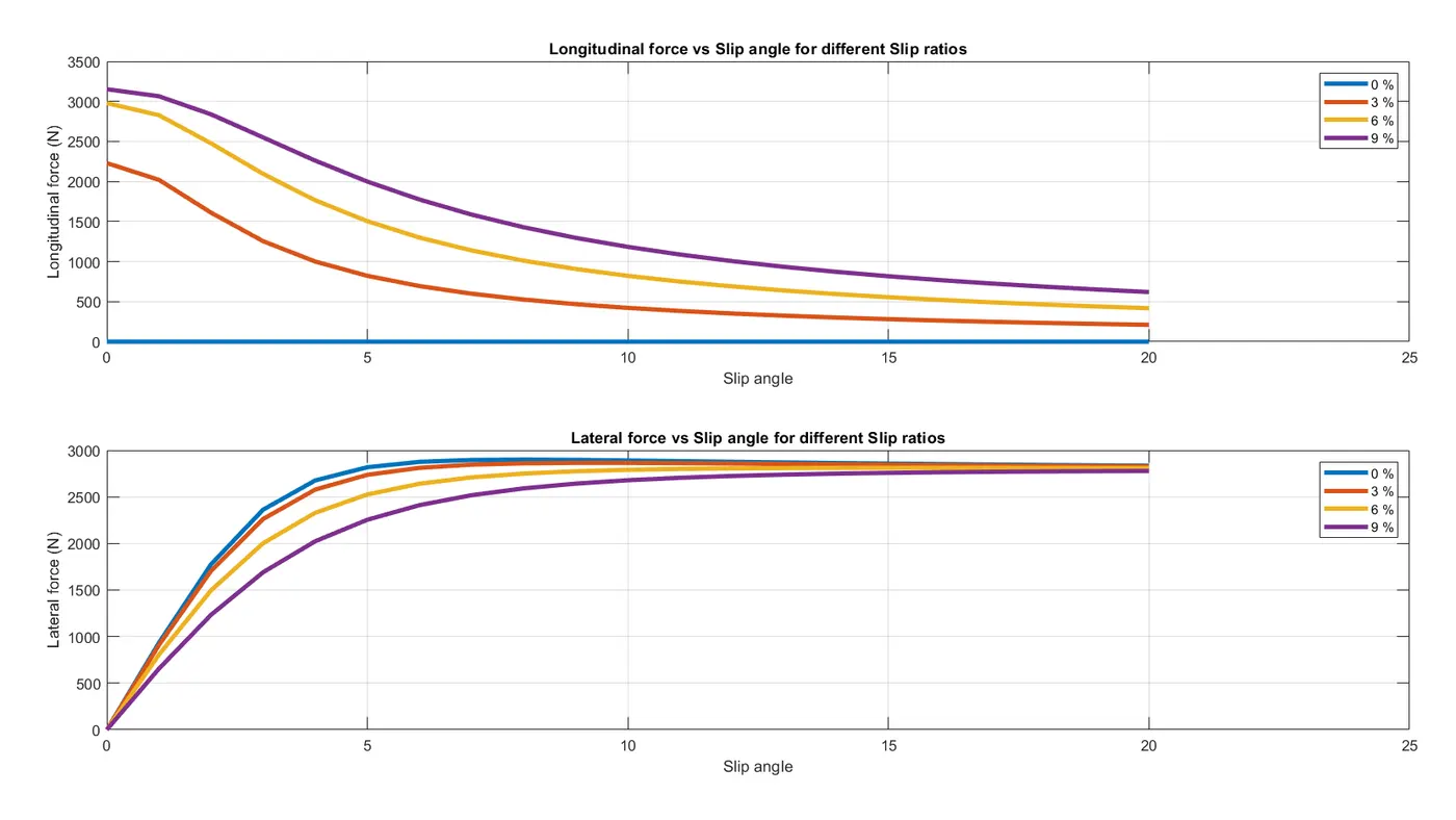
CONCLUSION: From the above results, we can infer that:

1.

- The highest peak longitudinal force occurs at zero slip angle.

- By increasing the slip angle, the longitudinal force decreases significantly within the tire.

- Due to the combined slip, the longitudinal force decreases with an increase in slip ratio and the tire saturates eventually.

- There is zero lateral force occurring at zero slip angle (i.e. free rolling case)

- By increasing the slip angle, the traction force increases significantly within the tire, thus reducing it's cornering capability.

- Due to the combined slip, the lateral force decreases with an increase in slip ratio and the tire saturates eventually.

2.

- There is zero longitudinal force occurring at zero slip ratio (i.e. free rolling case).

- By increasing the slip ratio, the longitudinal force increases significantly within the tire.

- Due to the combined slip, the longitudinal force decreases with an increase in slip angle and the tire saturates eventually.

- The highest peak lateral force occurs at zero slip ratio.

- By increasing the slip ratio, the traction force decreases significantly within the tire, thus reducing it's cornering capability.

- Due to the combined slip, the lateral force decreases with an increase in slip angle and the tire saturates eventually.