Combined Slip Brush Tire Model

AIM: To plot the combined slip brush tire model.

GIVEN DATA:

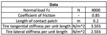
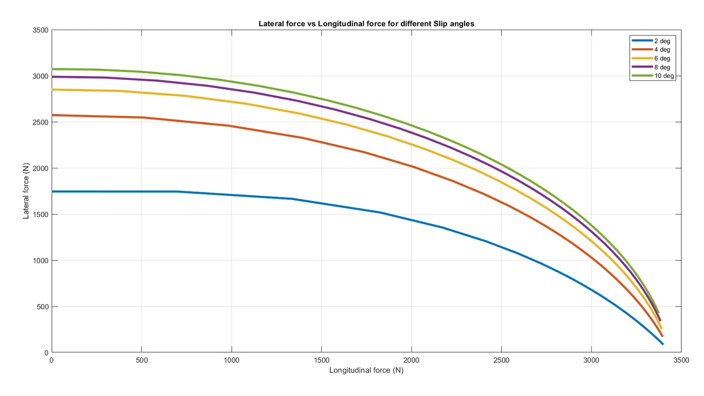
OBJECTIVE: To show the effect of slip angles on the longitudinal force vs lateral force relationship using:

- Slip angle (2 through 10 deg in increments of 2)

- Slip ratio range of 0 to 1 (or 0 to 100%)

GOVERNING EQUATION: The combined brush tire model is conceptualized in the following three zones;

1. Adhesion region:

Longitudinal force, `F_x = frac(C_s.s)(1-s)`

Lateral force, `F_y = frac(C_(alpha).s)(1-s)`

where;

`C_s = 1/2 . k_x . l_t^2` = Longitudinal stiffness (N/m^2)

`C_(alpha) = 1/2 . k_y . l_t^2` = Cornering stiffness (N/m^2)

`k_y` = stiffness (N/m^2)

`l_t` = Length of contact patch (m)

`s` = Slip/Skid ratio

2. Critical point:

Critical length, `l_c = frac(mu_p . F_z . (1-s) . l_t)(2 sqrt((C_s.s)^2 + (C_(alpha).tan(alpha))^2)`

where;

`mu_p` = Peak road-tire friction coefficient

`F_z` = Normal load (N)

3. Sliding (Large Excitation) region:

Longitudinal force, `F_x = frac(mu_p.F_z.C_s.s)(sqrt((C_s.s)^2 + (C_(alpha).tan(alpha))^2)) . [1 - frac(mu_p.F_z.s)(4.sqrt((C_s.s)^2 + (C_(alpha).tan(alpha))^2))]`

Lateral force, `F_x = frac(mu_p.F_z.C_(alpha).tan(alpha))(sqrt((C_s.s)^2 + (C_(alpha).tan(alpha))^2)) . [1 - frac(mu_p.F_z.s)(4.sqrt((C_s.s)^2 + (C_(alpha).tan(alpha))^2))]`

THEORY:

• So far, longitudinal and lateral slip were dealt with in isolation (pure cornering or pure tractive)
• In reality, these forces occur simultaneously during vehicle maneuvers like brake in turn and trailing throttle cornering
• Therefore a tire model must be able to deal with combined tractive and cornering forces, a situation known as comprehensive slip

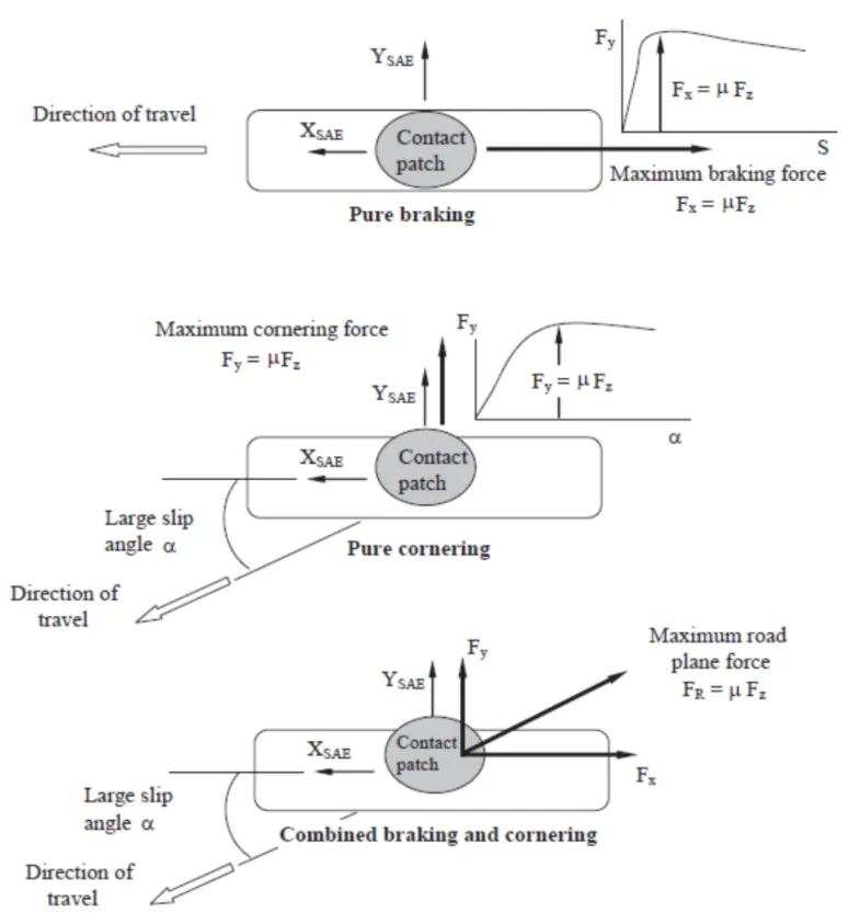
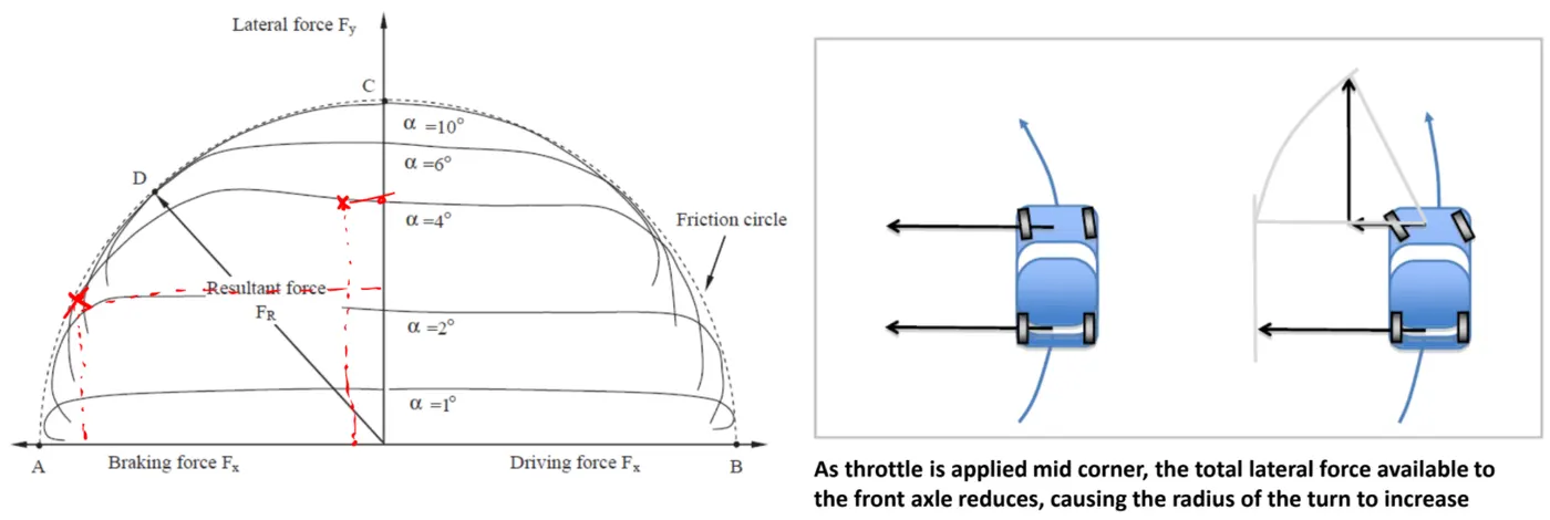
• The peak value of the resultant cornering and tractive forces is governed by a curve of radius μFz
• This curve is known as the friction circle or the friction ellipse as some tires have more capability in traction or cornering

Combined Slip - ABS and TC:

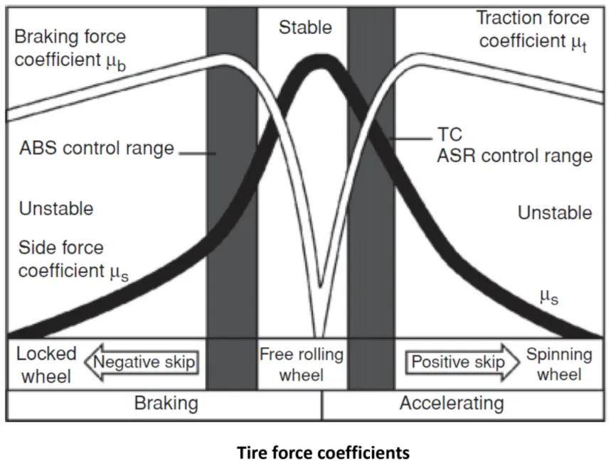
Anti-lock brake systems and traction control systems aim not only to avoid wheel lockup or spin but also to maintain wheel slip near an optimal value, which achieves maximum possible tire longitudinal forces and in the meantime, avoids a significant reduction in lateral forces.

SOLUTION:

Programming Language: MATLAB

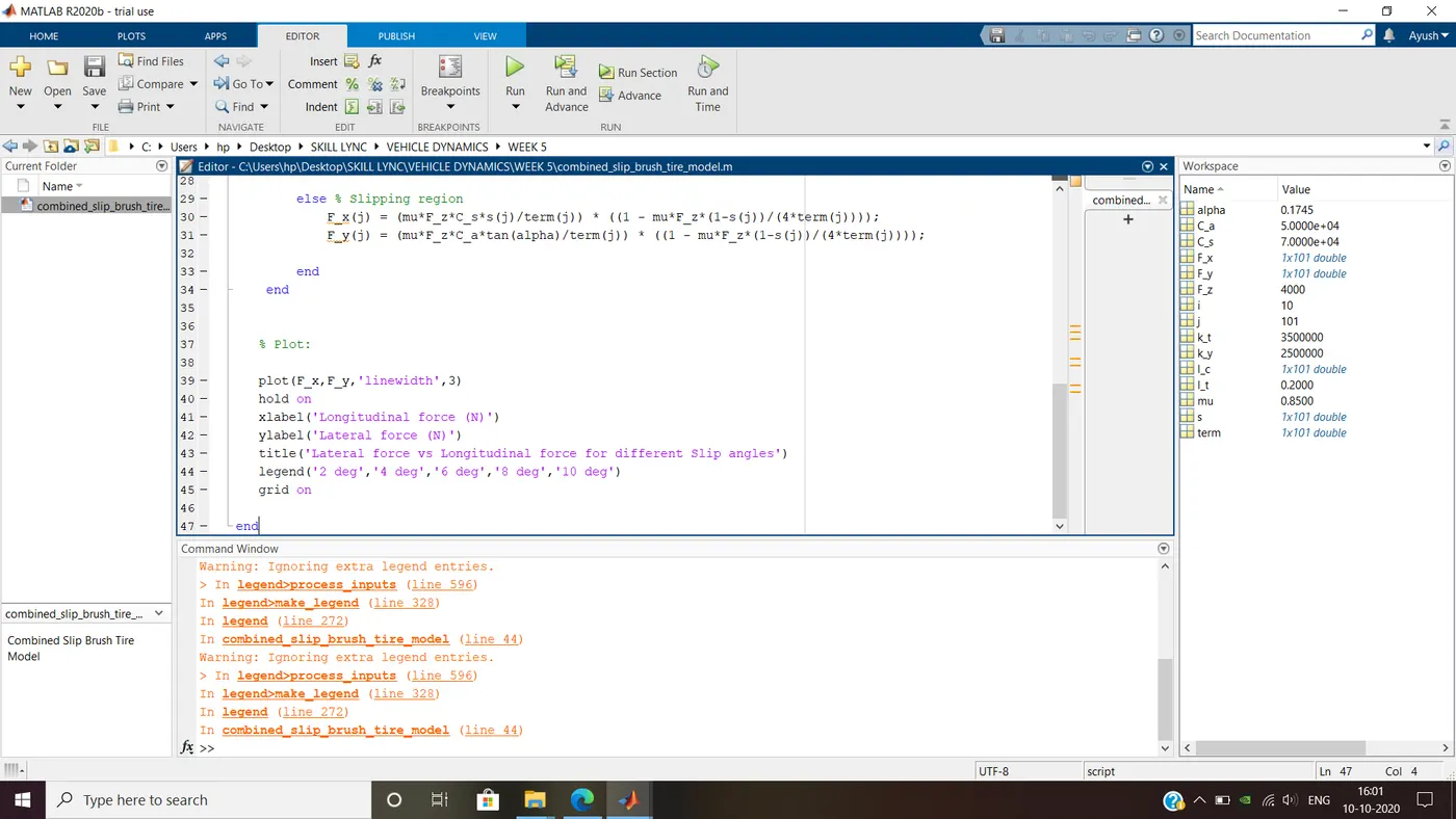
Code:

% Combined Slip Brush Tire Model

% Input data:

F_z = 4000;   % Normal force (N)
mu = 0.85;    % Peak road-tire friction coefficient
l_t = 0.2;    % Length of tire contact patch
k_t = 3.5e6;  % Tire tangential stiffness (N/m^2)
k_y = 2.5e6;  % Tire lateral stiffness (N/m^2)

% Solution:

C_s = 0.5*k_t*l_t^2;
C_a = 0.5*k_y*l_t^2;  % Lateral stiffness (N)
  
for i=2:2:10
    alpha = i*pi/180;
    
    for j=1:101
        s(j) = (j-1)*0.01;
        term(j) = ((C_s*s(j))^2 + (C_a*tan(alpha))^2)^0.5;
        l_c(j) = mu*F_z*(1-s(j))*l_t / (2*term(j));   % Critical length
     
        if l_t <= l_c
            F_x(j) = C_s*s(j)/(1-s(j));
            F_y(j) = C_a*tan(alpha)/(1-s(j));
            
        else % Slipping region
            F_x(j) = (mu*F_z*C_s*s(j)/term(j)) * ((1 - mu*F_z*(1-s(j))/(4*term(j))));
            F_y(j) = (mu*F_z*C_a*tan(alpha)/term(j)) * ((1 - mu*F_z*(1-s(j))/(4*term(j))));
            
        end
    end
   
   
   % Plot:
   
   plot(F_x,F_y,'linewidth',3)
   hold on
   xlabel('Longitudinal force (N)')
   ylabel('Lateral force (N)')
   title('Lateral force vs Longitudinal force for different Slip angles')
   legend('2 deg','4 deg','6 deg','8 deg','10 deg')
   grid on
   
end

Output:

Plot:

CONCLUSION:

1. Due to the difference in magnitudes of tangential stiffness and lateral stiffness, the friction circle can be visualized as an ellipse instead of a circle.

2. Lateral force decreases with an increase in longitudinal force.

3. Lateral force is increased with higher slip angles.

---------------------------------------------------------------------------------------------------------------------------------------------------------------------------------------------------------------------------------------------------------------------------------------

GIVEN DATA:

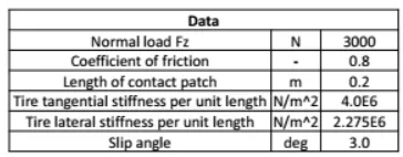
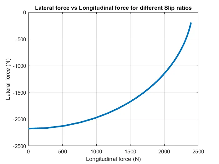
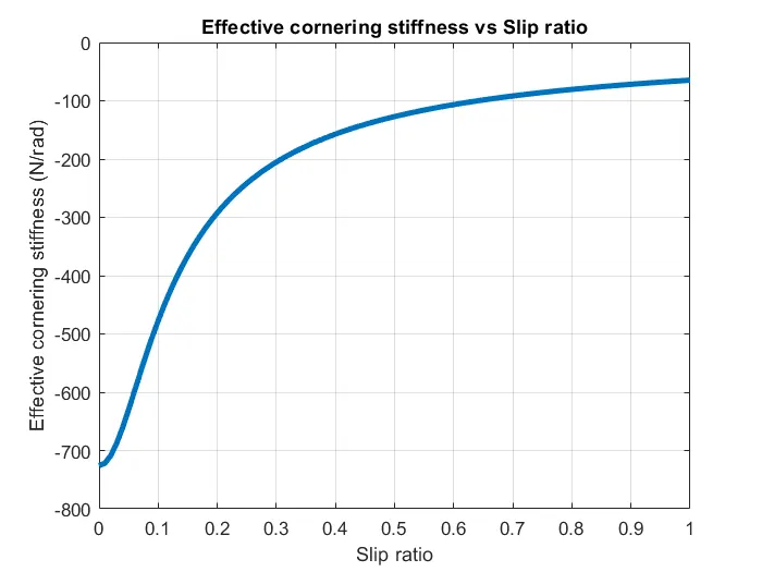
OBJECTIVE: To calculate the effective cornering stiffness using:

- Slip ratios (0, 0.15 and 1.0)

- Slip angle (3 deg)

GOVERNING EQUATION:

Effective cornering stiffness (N/rad), `C_(eff) = frac(F_y)(alpha)`

SOLUTION:

Programming Language: MATLAB

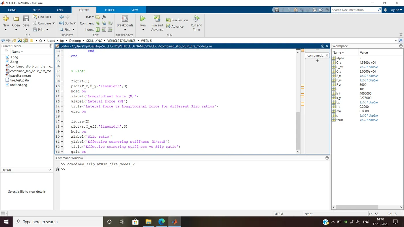
Code:

% Combined Slip Brush Tire Model - Different slip ratios and same slip angle

% Input data:

F_z = 3000;   % Normal force (N)
mu = 0.8;     % Peak road-tire friction coefficient
l_t = 0.2;    % Length of tire contact patch
k_t = 4e6;    % Tire tangential stiffness (N/m^2)
k_y = 2.275e6;  % Tire lateral stiffness (N/m^2)
alpha = 3     % Slip angle (degrees)


% Solution:

C_s = 0.5*k_t*l_t^2;   % Longitudinal stiffness (N)
C_a = 0.5*k_y*l_t^2;   % Cornering stiffness (N)
  
for i=1:101
        s(i) = (i-1)*0.01;   % Slip ratio
        term(i) = ((C_s*s(i))^2 + (C_a*tan(alpha))^2)^0.5;
        l_c(i) = mu*F_z*(1-s(i))*l_t / (2*term(i));   % Critical length
     
        if l_t <= l_c        % Adhesion region
            F_x(i) = C_s*s(i)/(1-s(i));
            F_y(i) = C_a*tan(alpha)/(1-s(i));
            C_eff(i) = F_y(i)/alpha; 
            
        else                 % Slipping region
            F_x(i) = (mu*F_z*C_s*s(i)/term(i)) * ((1 - mu*F_z*(1-s(i))/(4*term(i))));
            F_y(i) = (mu*F_z*C_a*tan(alpha)/term(i)) * ((1 - mu*F_z*(1-s(i))/(4*term(i))));
            C_eff(i) = F_y(i)/alpha;
            
        end
end


% Plot:
   
figure(1)
plot(F_x,F_y,'linewidth',3)
hold on
xlabel('Longitudinal force (N)')
ylabel('Lateral force (N)')
title('Lateral force vs Longitudinal force for different Slip ratios')
grid on
   
figure(2)
plot(s,C_eff,'linewidth',3)
hold on
xlabel('Slip ratio')
ylabel('Effective cornering stiffness (N/rad)')
title('Effective cornering stiffness vs Slip ratio')
grid on

Output:

The effective cornering stiffness for different slip ratios is given here: https://docs.google.com/spreadsheets/d/1oukCyADg4Y1BSVRiBRbnfJvTKK2crjiw4_bpvJn5xEc/edit?usp=sharing

Slip ratio	Effective cornering stiffness
0	-725.992940116735
0.15	-366.163561325828
1	-64.64656776231

Plot: