Braking and Motor Efficiency Plots

AIM : To study about brakes and breaking energy using MATLAB.

OBJECTIVES :

• For a defined driving cycle, calculate the energy required for braking.
• Why electric motor can’t develop braking torque at high speed similar to starting? How electric and mechanical brakes are coordinated?
• Make a MATLAB program which plots contour of given motor speed, torque and efficiency values.

1. For a defined driving cycle, calculate the energy required for braking.

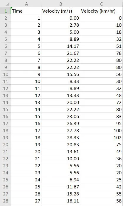
To calculate the energy required for braking, we will have to create our driving cycle first. We will create our driving cycle in an Excel Sheet.

Link to Excel Sheet : https://drive.google.com/file/d/1shEv1avFUgYb_7yAKrebfP49EtmKauIo/view?usp=sharing

The drive cycle is for 60 seconds with vehicle speed or velocity in km/hr converted to m/s which includes acceleration as well as deceleration of the vehicle where deceleration is considered as braking for calculation of energy.

Now we will read this drive cycle data in our MATLAB script.

clear all
close all
clc

%Reading the Drive Cycle Data
A = xlsread('W9 Drive Cycle.xlsx');

%Assigning Time and Velocity data to variables
T = A(:,1);
V = A(:,2);

M = 1200;  %Mass in kg

%Calculating the energy required for braking
for i = 1:(length(T)-1)
    if V(i)>V(i+1)
       E(i) = 0.5*M*(V(i+1)-V(i))^2;
    end
end

%Plotting
plot(T,V)
xlabel('Time(s)')
ylabel('Velocity(m/s)')
title('Drive Cycle')

%Displaying the total braking energy in command window
fprintf('The total energy required for braking is %.2f KJ',sum(E)/1000) 

Step-wise Explanation of the Code :

• The code starts with clear all, close all and clc where,

• ‘clear all’ command is used to clear the data stored in the workspace.
• ‘close all’ command is used to close all plots and figures.
• ‘clc’ command is used to clear the command window.

• Now to read the drive cycle data in MATLAB, we are going to use the xlsread command along with the appropriate file name and store it in a variable. We have to make sure that the excel file is present in MATLAB directory.
• Now we will assign the Time and Velocity data to the variables T and V from the Excel sheet. We will also define the mass of the vehicle.
• We will use the for loop to calculate the energy required for breaking along with an if loop wherein for every value of time, the corresponding value of velocity will be checked and if it’s a case of deceleration or breaking, then the braking energy will be calculated using the following formula,

`E=1/2 M(V_f-V_i )^2`

• Now we will plot the Drive cycle data for Time and Velocity using proper label and suitable title.
• To display the total braking energy through the drive cycle in the command window we will use the fprintf The %.2f command will display the calculated result upto 2 decimal places for the summation of the total energy divided by 1000 to get the answer in Joules.

RESULT :

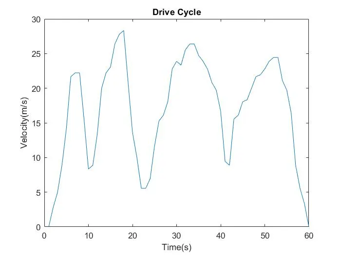
So according to the drive cycle, the deceleration of the vehicle is calculated and displayed in command window.

The total energy required for breaking is 250.32 KJ or 0.069 KWh.

2. Why electric motor can’t develop braking torque at high speed similar to starting?

Regenerative braking in EVs and HEVs adds some complexity to the braking system design. The fact that an electric motor can be used to convert kinetic energy back into electrical energy is an important feature of electric vehicles. As we know the torque equation is given by,

`T = F.r`

Where, T is torque of the motor, F is the force applied, r is the radius of the wheel; so during the starting conditions of the vehicle, the motor is at rest initially. As the throttle pedal is actuated, electric motor starts its working and a large amount of force is experienced at the wheel. As this force developed has negligible external resistance, almost all the applied power gets converted to torque and we get a higher starting toque at the wheels during starting.

Now under running condition or under vehicle’s performance in dynamic condition, the electric motor has some speed and momentum associated with it. At the same time during deceleration or when the brakes are applied at high speed, the force opposing the wheel or the motor is comparatively less than the force applied by the motor during forward motoring. As per the torque equation, the value of braking force decreases which decreases the braking torque developed. So the electric motor can’t develop braking torque at high speed similar to starting condition.

How electric and mechanical brakes are coordinated?

The braking force on the wheels is divided into two parts, regenerative braking force and mechanically frictional braking force. In an Electric vehicle, the traction motor must be controlled to produce the proper amount of braking force for recovering the kinetic energy as much as possible and, at the same time, the mechanical brake must be controlled to meet the braking force command from the driver. When the braking force demanded is less than the maximum braking force that the electric motor can produce, only electrically regenerative braking will apply.

When the commanded braking force is greater than the available regenerative braking force, the electric motor will operate to produce its maximum braking torque, and the remaining braking force is met by the mechanical brake system. The maximum regenerative braking force produced by an electric motor is closely related to the electric motor’s speed. At low speed, the maximum torque is constant. However, at high speed, the maximum torque decreases hyperbolically with its speed. Therefore, the mechanical brake torque at a given vehicle deceleration varies with vehicle speed.

3. Make a MATLAB program which plots contour of given motor speed, torque and efficiency values.

Contour plots are a way to show a three-dimensional surface on a two-dimensional plane. It graphs two predictor variables X Y on the y-axis and a response variable Z as contours. Contour lines commonly show altitude.

Now we will make a MATLAB program to plot contour of motor speed, torque and efficiency values where efficiency values will be the altitude or the Z axis. In order to plot this, we need the specifications of a motor. In this equation, We are assuming generic values for the specifications of the motor as well as for the losses that occur in the motor operation.

MATLAB Program :

clear all
close all
clc

%Defining Velocity and Torque values
Velocity = linspace(0,1000,100);
Torque = linspace(0,300,100);

%Loss Coefficients
kc = 0.18;            %Coefficient for Copper Loos
ki = 0.007;           %Coefficient for Iron Loss
kw = 0.000015;        %Coefficient for Windage Loss

%Creating 2D array for Velocity and Torque
[W,T] = meshgrid(Velocity,Torque);

%Calculating the Losses
cu_loss = kc*(T.^2);         %Copper losses
fe_loss = ki*W;              %Iron losses
win_loss = kw*(W.^3);        %Windage losses
con_loss = 20;               %Constant motor losses

%Power Calculations
Output_Power = (W.*T);
Input_Power = (Output_Power) + (cu_loss) + (fe_loss) + (win_loss) + (con_loss);

%Efficiency Calculation
E = ((Output_Power)./(Input_Power));

%Defining value range for Efficiency Curve
V = linspace(0.78,0.98,10);

%Plotting Contour for Speed, Torque and Efficiency
contour(W,T,E,V)
colorbar
xlabel('Angular Velocity (rad/s)')
ylabel('Torque (Nm)')
zlabel('Efficiency')
title('Speed, Torque and Efficiency Characteristics of Motor')

At first, we will start by defining the values of Velocity and Torque by using linspace command to generate linearly spaced vectors or values. These arrays are then used to create 2D grid coordinates using the meshgrid command. These coordinates will help in the creation of contour plot. In order to find the efficiency of the motor, we need to consider various losses that occur in the motor’s operation.

The major sources of loss in the electric motor can be divided into four main types, as follows,

• Copper Losses – These are caused by the electrical resistance of the wires (and brushes) of the motor. This causes heating, and some of the electrical energy supplied is turned into heat energy rather than electrical work. They are given by,

Copper Losses = `k_c T^2`

Where T is torque and k_c is a constant depending on the resistance of the brushes and the coil, and also the magnetic flux.

• Iron Losses – They are caused by magnetic effects in the iron of the motor, particularly in the rotor. The rate of change of magnetic flux is directly proportional to the speed of the rotor and it is given by,

Iron Losses = `k_i ω`

Where w is the speed of the rotor and k_i is constant depends on the way the magnetic field is provided.

• Friction and Windage losses – There will of course be a friction torque in the bearings and brushes of the motor. The rotor will also have a wind resistance, which might be quite large if a fan is fitted to the rotor for cooling. The friction force will normally be more or less constant. However, the wind resistance force will increase with the square of the speed. To get the power associated with these forces, we must multiply by the speed. So,

Windage Losses = `k_w ω^3`

• Constant motor losses – These losses occur even if the motor is totally stationary, and vary neither with speed or torque. The letter C is used to designate these losses.

It is useful to bring together all these different losses into a single equation that allows us to model and predict the losses in a motor. So we have,

Total Losses = `k_c T^2+k_i ω+k_w ω^3+C`

The motor efficiency is given as,

`η_m=(Output Power)/(Input Power)=(P_(o))/P_i`

Where,

`P_o=Tω`

`P_i=P_out+k_c T^2+k_i ω+k_w ω^3+C`

Now we will insert all these equations and constant coefficients in the MATLAB script file.

Then we will calculate in the output power and input power to calculate the efficiency with the help of these formulas. We will also define the value range for the efficiency curve in variable V which will act as corresponding values for Z axis by using linspace command.

Now we will plot contour of motor speed, torque and efficiency values with contour command with suitable label and title. The colorbar command displays a vertical colorbar to the right of the current axes or chart. Colorbars display the current colormap and indicate the mapping of data values into the colormap.

RESULT :

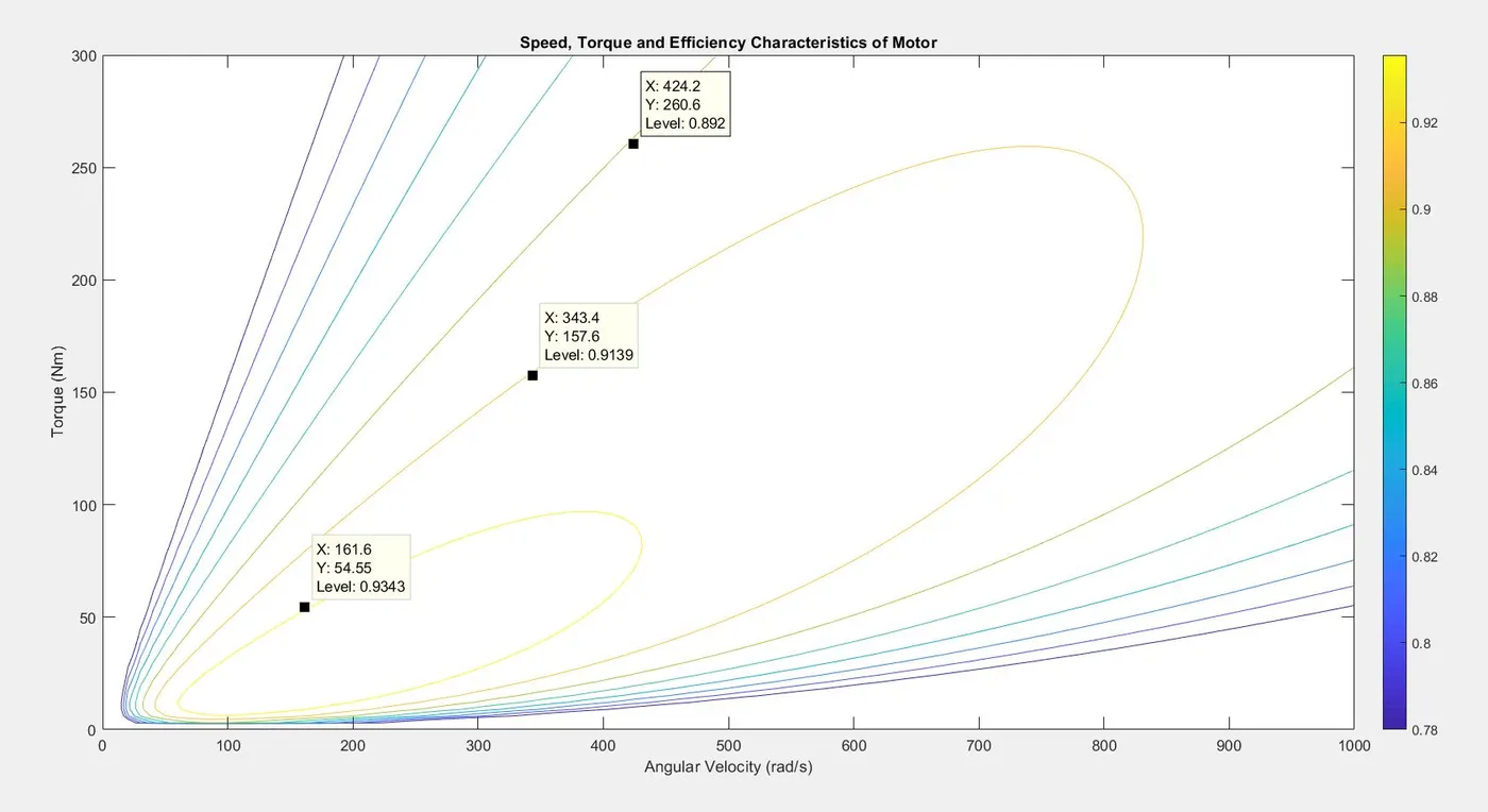
As we can see in the above plot, the contour of motor speed, torque and efficiency values have been plotted. Any point on the plot gives its corresponding values by using data cursor.

If we want to display the actual efficiency values on the contour plot, we can change the contour command for plotting as follows,

[C,h] = contour(W,T,E,V)
clabel(C,h);

This command returns the contour matrix C containing the data that defines the contour lines, and the Contour object h. The clable function uses the contour matrix to label the contour lines.

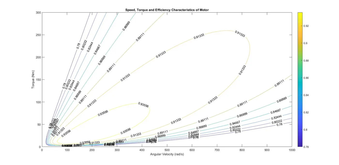
In the above plot, the efficiency values are visible.