Basics of Probability and Statistics

Now to understand the difference in the formula of variance for population size and sample, first understand the purpose of sample and population of data. Lets just say we wish to find out average hours of watching TV per day in a country. Now to find out this average one would nedd to go door to door to get the data for every human being in the country. And then take out its average. But this is easier said than done. Doing this will encounter two problems:-
1) Its too humongous a task to carry out for which the cost will be extortionate and the government or the institution, to whom this concerns, will not allocate outragiously high funds for this task
2)It will take a lot of amount of time to carry out this operation so by the time the data is available for mean average calculation, the data itself becomes old
So to counter this Samples are taken out of a population to estimate the characteristics of the population. Now the formula for mean and variance for the population is as follows:

N=Population size n=Sample size
X=member of the population
x=member of Sample
`mu`=mean of the population
`bar x`=mean of the sample
`sigma^2`=Variance of the population
`s^2`=Sample Variance
Population mean=`mu=(sum_(i=1)^N X_i)/N`
Population variance=`sigma^2=(sum_(i=1)^N( X_i-mu)^2)/N`
Population mean gives a central tendency of the data and variance tells about the overall spread of the data.

Now to estimate Mean and Variance of the population, mean and variance of the Sample is found out. The formula is as follows:
Sample mean=`bar x=(sum_(i=1)^n x_i)/n`
Sample variance=`s^2=(sum_(i=1)^n( x_i-bar x)^2)/(n-1)`

So the confusion happens when we see the difference in the formula for population variance and sample variance. The populaion variance seems right but sample formula does not sit right with the intuition. Lets first understand an important difference:-
That Sample variance is not variance of the data set present in the Sample but an estimate of the variance of the population from where it is derived. So Sample Variance does not tell you about variance of the Sample itself but the population.

Note:- It is common misconception or it is easy to misinterpret that with one sample, population'a characteristics can be appraised. Once sample size has been decided, only after a lot of samples can proper estimation be done about the population. Data from a single sample is untrustworthy regardless of its accuracy. The more the number of samples, the better the appraisal of the population data.

But the reason for the n-1 instead of n will be established in the following study done in matlab.

Step 1:- Generation of Population data

Using matlab 1000 random numbers (all integers) are chosen from the interval [1,100]. This is done using randi function to get 1000 numbers (numbers may be repeated) between 1 and 100. These numbers once generated are stored by the matlab function as text file to be accessed on a later stage to get samples. the code is as follows:-

clear all
close all
clc
Population_upper_limit=100;
Population_size=1000;
P=randi(Population_upper_limit,1,Population_size);
f1=fopen('D:DocumentsSkill lyncMachine Learning and AISample_variance_projectPOPULATION.txt','w');
for i=1:length(P)
fprintf(f1,'%3.0fn',P(i));
end
fclose(f1)

Step 2:- Generation of a sample

So a code for a function is written which will take population array and sample size as input and give Sample array as output. In this an array is generated of number of elements equal to sample size between 1 and population size(in this case 1000) using randperm function. randperm function returns an array of random numbers between 1 and upper limit of specified size and any element in this array is not repeated. So the upper limit is set as population size an specified size is set as sample size. These numbers from rand perm are used to store elements of population array ,which have position index same as array generated by randperm, in sample array. This sample array is taken as output.

function [S]=Sample_generator(P,Sample_Size)
Population_size=prod(size(P));
sel=randperm(Population_size,Sample_Size);
for i=1:length(sel)
S(i)=P(sel(i));
end
end

Step 3: Writing code for the main study

1st study: first population distribution will be observed in the form of histogram between 1 and 100. Second a formula of sample variance will be tested by
`s^2=(sum_(i=1)^n( x_i-bar x)^2)/(n-a)`
So if a=0, the formula becomes similar to the formula of variance of the population and if a=1, the formula becomes the one accepted in mathematics today. And the variance formula behaviour is checked for a=2.
So the idea is captured with Sample variance vs Sample mean scatter plot. So a dot or star '*' signifies one sample and many such stars signify variance and mean from many samples. Sample size is fixed as 10 and number of samples to be taken are 100. In the graph a marker of population variance and population mean is given to give an idea of orientation of Sample data with respect to population data.
The code is as follows:-

clear all
close all
clc
%Open population generator to generate a population, if already done so
% then ignore this message
format long
%Reading data from generated population data
f1=fopen('D:DocumentsSkill lyncMachine Learning and AISample_variance_projectPOPULATION.txt','r');
P=fscanf(f1,'%f',[1 inf]);
fclose(f1)

%Characteristics of the population data
Population_size=prod(size(P));
mean_POPULATION=mean(P);
%Variance of population
sum=0;
for i=1:length(P)
sum=sum+(P(i)-mean_POPULATION)^2;
end
variance_POPULATION=sum/Population_size;
standard_deviation=sqrt(variance_POPULATION);
figure(1)
histogram(P,50)
xlabel('variable value')
ylabel('Frequency')
text_mean=sprintf('Population Mean=%3.3f,Variance=%3.3f and Standard Deviation=%3.3f',mean_POPULATION,variance_POPULATION,standard_deviation);
title({'population distribution',text_mean})
figure(2)
%Sample select
Sample_size=10;
number_of_samples=100;
for j=1:number_of_samples
[S]=Sample_generator(P,Sample_size);
    %Sample mean
     Sample_mean=mean(S);
    %Sample Variance
    sum1=0;
for i=1:length(S)
sum1=sum1+(S(i)-Sample_mean)^2;
end
a=1;
variance_Sample=sum1/(Sample_size-a);

%sprintf('%3.3f',mean_POPULATION)
%sprintf('%3.3f',variance_POPULATION)
%sprintf('%3.3f',Sample_mean)
%sprintf('%3.3f',variance_Sample)

study_mean(j)=Sample_mean;
study_variance(j)=variance_Sample;
end
plot(study_mean,study_variance,'*');
hold on
plot([mean_POPULATION mean_POPULATION],[0 max(study_variance)],'--');
hold on
plot([0 max(study_mean)],[variance_POPULATION variance_POPULATION],'--');
xlabel('Sample Mean')
ylabel('Sample Variance')
legend('Per sample data cluster','Population mean','Population Variance')
title('Sample Variance vs Sample Mean')

So the histogram of population distribution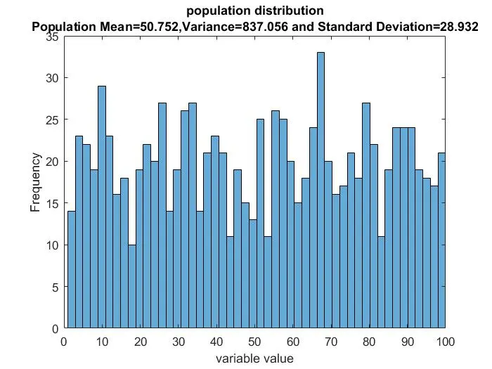

For Sample size=10, a=0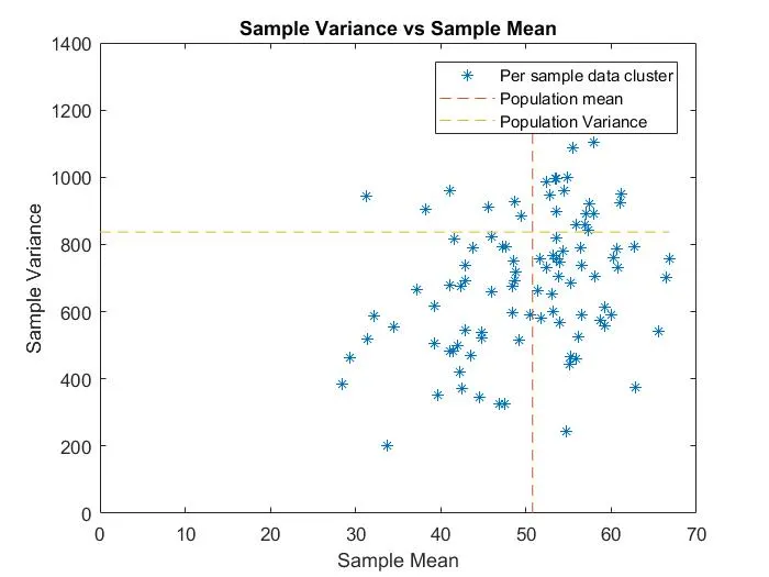


For Sample size=10, a=1
(The accepted mathematical formula for variance)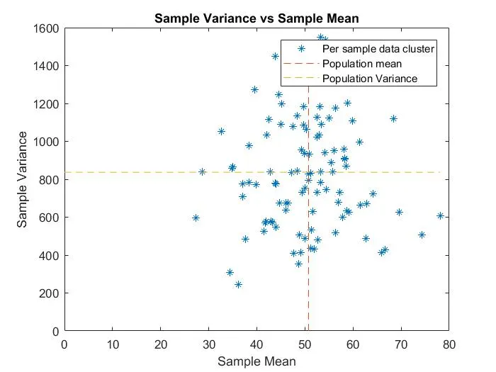


For sample size size=10 and a=2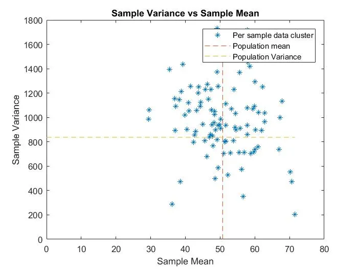


Lets make the sample a little bigger; n=50 with a=0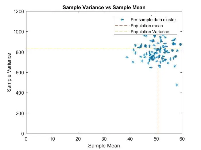


Now as it can be seen from all the graphs, the (Sample mean,Sample variance) data points hover around the (Population mean,Population variance) point. The only difference is the closeness or sparseness of the data. So when n=10 and a value is changed from 0 to 2, there are slight observations made from the cluster of data for each graph. So when a=0, the overall data centrally seems to be lower than population data point. So a=0, leads to undrestimation of data while when a=2, the central point of the that is slightly above the population data point and therefore a=2, formula overestimates the population data point. But when a=1, the sample data centrally is very close to population data point. This was verified by taking an average of the respective data points and checking it with population data values.
Then an effect was observed by increasing the sample size, it was observed the clusters came considrably closer to population data point.

but the idea is still not that clear. A further investigation is done to do so

2nd Study:-
So I decided to make an array of Variance for a sample ranging from -1 to 3 and do this for a specific number of samples. And when I am doing this, I calculate average Variance for the current sample and variances calculated for samples previously. And this is done for each value of a. Simultaneously a marker is made for population variance to see at which value of a does the average variance becomes equal to population variance.
The code is as follows

clear all
close all
clc
%Open population generator to generate a population, if already done so
% then ignore this message
%Reading data from generated population data
f1=fopen('D:DocumentsSkill lyncMachine Learning and AISample_variance_projectPOPULATION.txt','r');
P=fscanf(f1,'%f',[1 inf]);
fclose(f1)

%Characteristics of the population data
Population_size=prod(size(P));
mean_POPULATION=mean(P);
%Variance of population
sum=0;
for i=1:length(P)
sum=sum+(P(i)-mean_POPULATION)^2;
end
variance_POPULATION=sum/Population_size;
standard_deviation=sqrt(variance_POPULATION);
histogram(P,50)
xlabel('variable value')
ylabel('Frequency')
text_mean=sprintf('Population Mean=%3.3f,Variance=%3.3f and Standard Deviation=%3.3f',mean_POPULATION,variance_POPULATION,standard_deviation);
title({'population distribution',text_mean})
%a values
a=-1:0.1:3;
%Sample select
Sample_size=10;
number_of_samples=350;
sum2=zeros(1,length(a));
for k=1:number_of_samples
[S]=Sample_generator(P,Sample_size);
Sample_mean=mean(S);
%Sample Variance
sum1=0;
for i=1:length(S)
sum1=sum1+(S(i)-Sample_mean)^2;
end
for i=1:length(a)
variance_Sample(i)=sum1/(Sample_size-a(i));
end
sum2=variance_Sample+sum2;
avg_variance=sum2./k;
plot(a,variance_Sample,'g')
hold on
plot(a,avg_variance,'r')
hold on
plot([a(1) a(end)],[variance_POPULATION variance_POPULATION],'--')
%to find a at which the average curve has population variance value
error=0;
pr=1;
for j=1:length(a)
error_old=error;
error=abs(avg_variance(j)-variance_POPULATION);
if error_old>error
pr=j;
end
end
if avg_variance(pr)>=variance_POPULATION
    if pr==1
    ap=a(pr);
    else
    ap=a(pr-1)+(a(pr)-a(pr-1))*((variance_POPULATION-avg_variance(pr-1))/(avg_variance(pr)-avg_variance(pr-1)));
    end
else
    if pr==length(a)
    ap=a(pr);
    else
    ap=a(pr)+(a(pr+1)-a(pr))*((variance_POPULATION-avg_variance(pr))/(avg_variance(pr+1)-avg_variance(pr)));
    end
end
%end calculation
plot([ap ap],[0 variance_POPULATION])
text1=sprintf('a=%f with Avg Var = Pop. Var',ap);
xlabel('a')
ylabel('Variance')
legend('Variance of current sample','Average Variance of all the samples till now','Population Variance',text1)
text=sprintf('Sample number=%f',k);
title({'Variance behaviour over increase in sample number',text});
axis([a(1) a(end) variance_POPULATION-200 variance_POPULATION+200])
hold off
pause(0.01)
end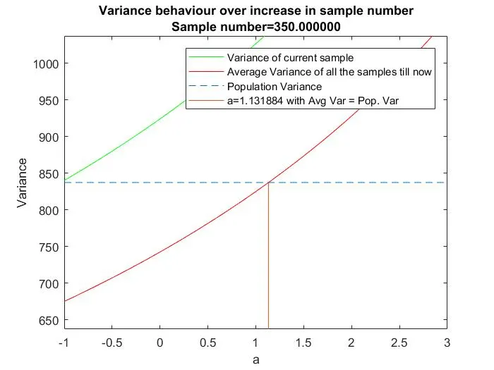

This code can be repeated for various values of sample sizes for many samples as possible. It will be found that the a value where the Sample variance will tend to oscillate about 1. This is true for 350 samples or 500 or even 1000 samples. It seems that putting a=1 gets the value of variance very close to population variance. Another observation that can be made is that when the formula is with a=0 (normal population variance like formula), the estimate of population variance by sample variance is grossly underestimated and while taking a value as 2, overestimates the population variance. Only a value equal to one closely estimates population variance.

Lets do one more study: This time we will assume that we are not aware of the sample variance formula and to estimate variance of the population, we will assume the same formula of population variance for sample variance.
So the formula for the Sample variance is:-
`s^2=(sum_(i=1)^n( x_i-mu)^2)/n`
The study will be done as follows: Different sample sizes will be selected and each sample size will be tested by taking specific sample number from population (in this case 500). And for each sampe size with average variance is calculated using the formula above and plotted as a bar graph. But in this case average variance value is not plotted against sample size but the ratio of average sample variance and population variance i.e`(avg(s^2))/sigma^2 *100`
as percentage values.
Then an interesting behaviour is observed and to understand this behaviour a line plot is graphed in the same figure of (Sample size -1)/sample size or `(n-1)/n` multiplied by 100 to make the fraction as percentage. This fraction value is plotted against sample size and interesting behaviour manifests itself.
The code is as follows

clear all
close all
clc
%Open population generator to generate a population, if already done so
% then ignore this message
%Reading data from generated population data
f1=fopen('D:DocumentsSkill lyncMachine Learning and AISample_variance_projectPOPULATION.txt','r');
P=fscanf(f1,'%f',[1 inf]);
fclose(f1)

%Characteristics of the population data
Population_size=prod(size(P));
mean_POPULATION=mean(P);
%Variance of population
sum=0;
for i=1:length(P)
sum=sum+(P(i)-mean_POPULATION)^2;
end
variance_POPULATION=sum/Population_size;

%Sample select
number_of_samples=500;
Sample_Size=[2 4 6 8 10 15 20 30 50];
for k=1:length(Sample_Size)
Sample_size=Sample_Size(k);
for j=1:number_of_samples
[S]=Sample_generator(P,Sample_size);
    %Sample mean
     Sample_mean=mean(S);
    %Sample Variance
    sum1=0;
for i=1:length(S)
sum1=sum1+(S(i)-Sample_mean)^2;
end
a=0;
variance_Sample=sum1/(Sample_size-a);

%sprintf('%3.3f',mean_POPULATION)
%sprintf('%3.3f',variance_POPULATION)
%sprintf('%3.3f',Sample_mean)
%sprintf('%3.3f',variance_Sample)

study_mean(j)=Sample_mean;
study_variance(j)=variance_Sample;
end
study_avg_sample_mean(k)=mean(study_mean);
study_avg_sample_variance(k)=mean(study_variance);
end
bar(Sample_Size,study_avg_sample_variance*(100/variance_POPULATION));
hold on
plot([0 max(Sample_Size)],[100 100],'--');
hold on
predicted_output=100*((Sample_Size-1)./Sample_Size);
plot(Sample_Size,predicted_output);
xlabel('Sample Sizes')
ylabel('Average Sample Variance/Population Variance');
legend('Ratio value','Population Variance marker','Plot of (sample size -1)/sample size')

The plot is as follows:-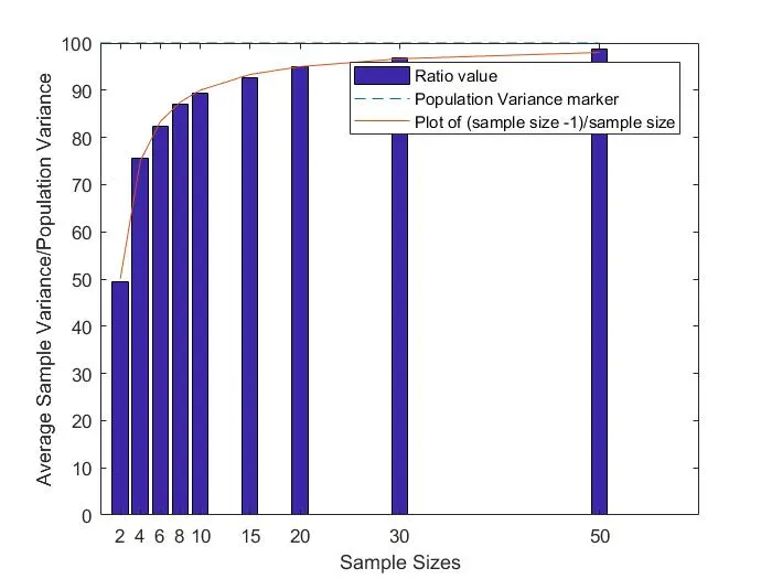

Population variance marker is denoted by 100 percent. It is observed as sample size increases, the average variance gets closer to population variance. But its important to look (n-1)/n plot and tips of the bar graphs for a sample size. It is observed that the value of (n-1)/n and average variance (by the assumed formula) seems to approximately coincide. And the most important thing is that these results are repeatable and reproduceable. No matter what is the population or population size, if the number of samples taken are sufficient, this is the kind of behaviour that is observed. Its really interesting to see (n-1)/n curve so closely fitting with the respective average variance values.
So from the above data it is found that for a Sample size n
`s^2/sigma^2~~(n-1)/n`
Lets take both of them as equal
`s^2/sigma^2=(n-1)/n`
Then further simplifying it, we get
`sigma^2=(n/(n-1))*s^2`
So if variance of the population has to be estimated, the above expression has to be enforced. But in this case, the formula for Sample variance is known, which is
`s^2=(sum_(i=1)^n( x_i-mu)^2)/n`......(Assumed for the time being)
substituting in the derived expression
`sigma^2=(n/(n-1))*(sum_(i=1)^n( x_i-mu)^2)/n`
further simplifying, we get
`sigma^2=(sum_(i=1)^n( x_i-mu)^2)/(n-1)`
Do not confuse how the above formula has `sigma^2`instead of`s^2`written. Remember the end objective of the formula is to estimate the variance of the population from the data present in the sample. But since the data belongs to the sample so the above corelation of sampe data to population variance is termed as Sample variance and the above expression is put in place with the said name as
`s^2=(sum_(i=1)^n( x_i-mu)^2)/(n-1)`
Also remember the above formula proves effective only and only if the sample number of the same sample size are significant enough. Otherwise the formula is not trustworthy.

Stratified Sampling and Clustered Sampling
Stratified Sampling concerns with dividing a population into strata and then drawing equalling from all these stratas to form a sample via simple random sampling. In Cluster sampling a huge population which is inherently heterogeneous is divided into different clusters. These clusters must have almost same composition between themselves. Then any one or two clusters are selected or 'sampled' and then samples are drawn from the selected cluster or clusters. Remember that any selection that is hinted is done via simple random sampling i.e done without any bias. To understand cluster sampling, imagine molecules in a milk. Milk in itself is heterogeneous mixture. Now to check the milk one pours the milk in four glasses equally. So each glass signifies a cluster. Now select any glass for sampling (Done via simple random sampling). So use that glass to draw small samples to test it for fat composition or sweetness. Now it is understood that milk is heterogeneous but the degree of homogeneity is same for each glass or sample. So any properties estimated for a that milk in the glass will be the almost same for the entire milk. Lets expound on both these methods a little more:-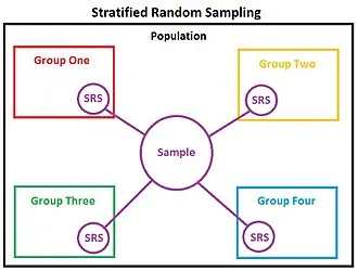

This image has been taken from wikipedia which explains best what stratified sampling. These Group 1,2,3 and 4 represent stratas. Imagine one wishes to find out average health index of an Indian. So imagine sampling being done from group of people who are mostly young adults, So u will get higher health index overall (maybe). But this means that the result is skewed since citizens of a country from all ages, and since older and younger children were not taken account the estimate is faulty. So to counter this the entire population, which in this case is India, is divided into stratas such that these groups are mutually exclusive i.e. any member of the population belongs to one and one group only and collectively exhaustive i.e these groups account for each member of a population. So in this case the stratas are :
1)Group or Strata 1: Ages from new born to 12 years old (Children)
2)Group or strata 2: Ages from 13 years old to 18 years old (Adolescent)
3)Group 3: Ages from 18 years old to 30 years old (young adluts)
4)Group 4:Ages from 31 years old to 50 years old (middle age adults)
5)Group 5:Ages from 51 to 65 years old (later stage adults)
6)Group 6:Ages above 65 years old (old people)
So there are 6 groups formed, so now to form a sample I will draw 2 members from each of these groups to form a sample of 12 members and then take reading of health index (it means reading of cholesterol, hemoglobin, fat content & BMI). So repectedly taking sample size of 12 the way indicated will insure overall appraisal of the population. Lets just say that the researcher finds out that there can be significant change in health index readings between woman, men and transgender in a particular age echelon. So then there can be sub-stratas as well forming woman, men and transgender. So in this case 6 groups and 3 sub groups and if a member of each group and sub group has to be accounted for then the minimum size of a sub group is 6 * 3 ie 18.

Clustered sampling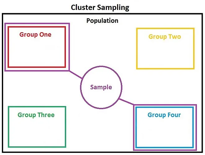

Cluster sampling is done when the population size is too large and heterogeneous. So the population is divided into clusters. The different between a cluster and a strata is that members of a strata will not share characteristics with another strata. For eg a when 6th grade classes in a school is divided into a group of boys as strata one and group of girls as strata two, one can notice that a boy will not be found in strata 2 or a girl will not be found in strata 1. But these stratas are not clusters. So a cluster will be when same 6th grade classes in school are divided into class sections A,B and C. So these clusters are in the basis of the sections in grade 6th in a school. So in Cluster or section A, a boy will be present and so will be existing in clusters or sections B and C. Same is true for girls as well. A cluster basically represents an entire population whereas a single strata cannot represent the entire population. That can be realized from the above example. So strata 1 (group of boys cannot represent the population of entire 6 th standard) but cluster 1 or section A can represent the entire population if the cluster is as heterogeneous as the entire population.

Cluster sampling is used which is heterogeneous over a area. Let us assume that there are three streets A,B,C and D. People living in those streets buy their vegetabes from a single market place in the neighbourhood. So its natural to assume that heterogeneity will be the same among all the streets. Lets just say I wish to find out the average age of a person buying vegetable from that neighbourhood, so its foolsome to go and check the age of every person that comes to the market. It may be possible that people may come from other neighbourhoods. So what I will do is that I will specify each street A,B,C and D as cluster 1,2,3 and 4 respectively. And then select 1 or 2 clusters out of these 4 clusters via simple random sampling, the way it is shown in the image. Then from these clusters I will start taking samples of people who go to the market and note down their age. After taking sufficient number of samples and realizing that the average has become steady with increase in number of samples, I will stop. And the steadied average value calculated from the set of samples will be taken as average age of the population i.e all the 4 streets.

Number of samples out of a population of size n

Lets imagine a population which has size n or has n number of members. And we wish to find out the number of different samples are possible. This means different combinations of different sizes that are possible. So lets just assume few things :-
1) Smallest size of a sample is 1
2) Biggest size of a sample is n
Lets just say for a sample size m, the number of combinations from n members of m size is `C_m^n`
So the formula for `C_m^n=(n!)/((m-1)!*m)`
So when m=1, the number of combinations=`C_1^n`
when m=2, the number of combinations is =`C_2^n`
.........
........
when m=n-1, the number of combinations is =`C_(n-1)^n`
when m=n, the number of combinations is =`C_n^n`

So the total number of combinations =(Combinations for sample size 1)+(Combinations for sample size 2)+........+(Combinations for sample size n-1)+(Combinations for sample size n)
=`C_1^n+C_2^n+......+C_(n-1)^n+C_n^n`
The same equation can be written as
Total number of combinations= `C_1^n*1^1+C_2^n*1^2+......+C_(n-1)^n*1^(n-1)+C_n^n*1^n`
Adding and substracting `C_0^n*1^0`
=`C_1^n*1^1+C_2^n*1^2+......+C_(n-1)^n*1^(n-1)+C_n^n*1^n+(C_0^n*1^0-C_0^n*1^0)`
Rearranging
=`C_0^n*1^0+C_1^n*1^1+C_2^n*1^2+......+C_(n-1)^n*1^(n-1)+C_n^n*1^n+(-C_0^n*1^0)`
Lets replace 1 with x
=`C_0^n*x^0+C_1^n*x^1+C_2^n*x^2+......+C_(n-1)^n*x^(n-1)+C_n^n*x^n+(-C_0^n*x^0)`...where x=1
There is a pattern that is observed and the above expression looks like Binomial theorem formula
i.e `(x+y)^n=C_0^nx^ny^0+C_1^nx^(n-1)y^1.......+C_(n-1)^nx^1y^(n-1)+C_n^nx^0y^n`
so if x=1, the formula will look like
`(1+y)^n=C_0^ny^0+C_1^ny^1.......+C_(n-1)^ny^(n-1)+C_n^ny^n`
if one looks in the expression for total combinations, one would see the above expression as a part of it. So substituting in the main formula we get
Total number of combinations=`(1+x)^n-C_0^n*x^0`
but we know that x=1 and `C_0^n=1`
So finally the total formula becomes,

Total number of possible different samples from a population of size n=`2^n-1`

The probability of drawing 2 jacks from a pack of card:-

Lets understand this problem. That a first card is drawn from a pack of 52 and then again a card is drawn from a pack of 51...(since a card was drawn previously).
So probability of getting a jack in the first time=`C_1^4*1/52`
Probability of getting a jack in the second time= `C_1^3*1/51`

Now the first event and the second event are independent events, so by multiplication rule of probability:
the probability of both the event occuring=P(A)*P(B)=`C_1^4*1/52*C_1^3*1/51`=`3/221`

Probability that both the numbers on two dices are same while rolling :-

Total number of possible outcomes when two dices are rolled=6*6=36
Total number of outcomes in which numbers on dices are same = 6
Possible permutations are:-
(1,1),(2,2),(3,3),(4,4),(5,5)&(6,6)....therefore 6
Probability=Total number of favourable event/ total number of possible outcome=`6/36=1/6`

Why standard deviation when variance can measure the dispersion in data

Standard deviation and variance both are measure for spread of data. So more the variance or standard deviation, more dispersed the data is. But there is a reason standard deviation is brought into picture. So imagine u have a data regarding distance traveled by a person every day. So some days he will travel to farthest corners of the city and on some days, he will not travel at all. So the data will be widely dispersed. When one asks what is the average distance travelled by that person per day for a month, the answer would be in km or metres. But if I ask how much is the data dispersed, one would say some number as variance but it will be a huge number since distances are squared i.e unit is in `km^2 or m^2`and therefore it looses physical significance. One cannot say that data was dispersed by 1600 km^2 when the maximum distance travelled is 98 km. So here physical significance is lost. But when I take square root of variance, I not only retain the dispersion measure but I also bring the physical meaning to the measure. So when I say standard deviation of 40 km, one can say that on an average his daily travel route varies by 40 km, which seems appropriate. Standard deviation is also used to find out how effectively has fluid mixed based upon data of temperature on the sureface of the fluid when a hot and cold fluids mix.