Basics of ML & AL Week 2 Challenge

Q1.
First business moment

The first business moment is the measure of central tendency

Mean or expected value, μ=∑x.P(x)

μ=1.4

Second business moment

The second business moment is the measure of dispersion. This is calculated by determining the variance of the given data

Variance,

σ²=∑(xi−μ)².P(x)

σ²=∑(xi−μ)².P(x)=1.84

Third business moment

The third business moment is the skewness. Skewness is a measure of the symmetry in distribution. The skewness for a normal distribution is zero. A positive skewness indicates that the size of the right-handed tail is larger than the left-handed tail and vice-versa

Sk=∑(xi−μσ)³.P(x)

Sk=∑(xi−μσ)³.P(x)=0.57

Fourth business moment

The fourth business moment is the kurtosis Kurtosis is a measure of the combined sizes of the two tails. It measures the amount of probability in the tails. The value is often compared to the kurtosis of the normal distribution, which is equal to 3.

If the kurtosis is greater than 3, then the dataset has heavier tails than a normal distribution (more in the tails). If the kurtosis is less than 3, then the dataset has lighter tails than a normal distribution (less in the tails).

Kt=∑(xi−μσ)⁴.P(x)−3

Kt=∑(xi−μσ)⁴.P(x)−3=2.04−3=−0.96

---

Q2.

Expected value: It is the Probability of an event multiplied by the amount of time the event happens.

A Probability Function defines the relative frequency outcomes of a random variable - the expected value.

In case of infinite number of Observations, it is very difficult to note each and every outcome. In such cases the probability of each outcome is determined using this probability. The formula is :

μ=∑x⋅P(x)

Simple Mean : In case of Finite number of Observations the sample mean is calculated by (Sum of all observations/number of observations) .

---

---

Q3.

Skewness: It is a measure of asymmetry of the probability density function of a real-valued random variable about its mean.

There are two types of Skewness:

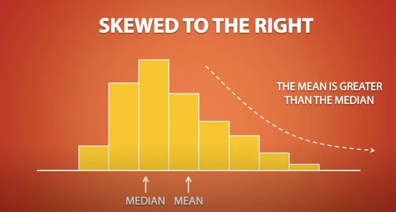
1) Positive or Right Skewness: When the tail on the right side of the distribution is longer or fatter. The mean and median will be greater than mode.

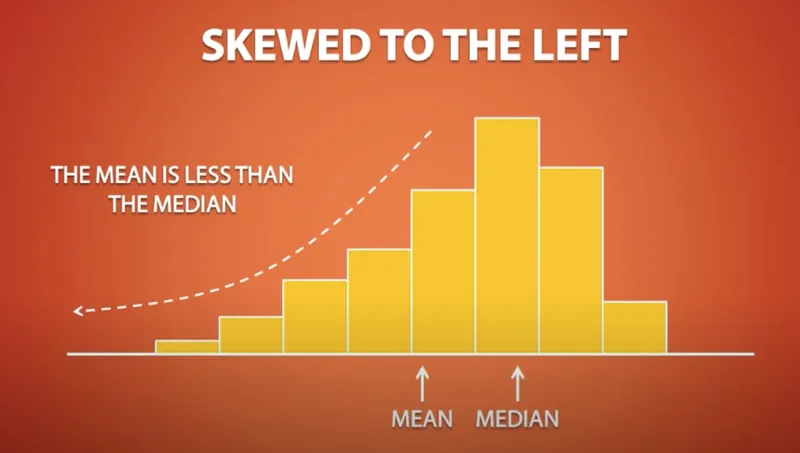
2) Negative or Left Skewness : When the tail on the left side of the distribution is longer or fatter. The mean and median will be less than mode.

i) If the skewness is between -0.5 and 0.5, the data are fairly symmetrical.

ii) If the skewness is between -1 and – 0.5 or between 0.5 and 1, the data are moderately skewed.

iii) If the skewness is less than -1 or greater than 1, the data are highly skewed.

Having skewness in the curve is not considered to be bad in the analysis, Skewness is the attribute to describe the distribution.

---

---

Q4.

Given data : mean(μ)=680 and standard deviation(σ)=31

a)P(X<711)

the Z-score for X$$=711:

Z=(711−680)/31=31/31=1

Now, we find P(Z<1). From the standard normal distribution table:

P(Z<1)≈0.8413

P(X<711)≈0.8413

b)P(X>740)

the Z-score for X=740

Z=(740−680)/31=60/31≈1.935

Now, we find P(Z>1.935). From the standard normal distribution table, we find $P(Z < 1.935)$P(Z<1.935), then subtract this from 1:

P(Z<1.935)≈0.9732

P(Z>1.935)=1−0.9732=0.0268

So, P(X>740)≈0.0268.

c) P(600<X<700)

We calculate the Z-scores for
X=600 and $X = 700$X=700:

For X=600:

Z=(600−680 )/31=−80/31≈−2.58

For X=700:

Z=(700−680)/31≈1.29

Now, we find P(−2.581<Z<1.29):

From the standard normal distribution table

P(Z<−2.581)≈0.0049

P(Z<1.29)≈0.9015

Thus, the probability is:

P(−2.581<Z<0.645)=0.9015−0.0049= 0.8966

So, P(600<X<700)≈0.8966.

d)P(X=720)

Z = (720-680)/31720-68031

Z = 1.29

The Probability of X = 720 is equal to the area under X = 720 which is very small. we need to subtract area on the left as well as the right side of the curve from the total area.

Therefore P(X = 720) = 0

---

---

Q5.

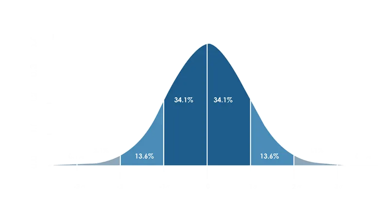
The curve shown in the figure represents a normal distribution. The peak of the curve divides the curve and the area is symmetric about the y-axis with the mean or expected value located at the origin. The right side of the curve is divided using the standard deviation as follows:

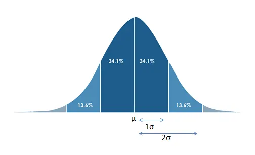
The area under the curve between the mean and 1 standard deviation is 34.1% of the total area. This means that 34.1% of the outcomes lie in this region.

Also, the area between μ+1σandμ+2σ${\displaystyle \mu +1\sigma \text{and}\mu +2\sigma }$ is 13.6% of the total area