Basics of ML & AL Week 2 Challenge
1)Calculate all 4 business moments using pen and paper for the below data set?
Business Moment - Mean:
μ=∑(Xi⋅P(X))μ=∑(Xi⋅P(X))
μ=(0×0.35)+(1×0.25)+(2×0.15)+(3×0.15)+(4×0.10)μ=(0×0.35)+(1×0.25)+(2×0.15)+(3×0.15)+(4×0.10)
μ=0+0.25+0.30+0.45+0.4μ=0+0.25+0.30+0.45+0.4
μ=1.4μ=1.4
Business Moment - Variance:
σ2=∑(Xi−μ)2⋅P(X)σ2=∑(Xi-μ)2⋅P(X)
σ2=(0−1.4)2⋅0.35+(1−1.4)2⋅0.25+(2−1.4)2⋅0.15+(3−1.4)2⋅0.15+(4−1.4)2⋅0.10σ2=(0-1.4)2⋅0.35+(1-1.4)2⋅0.25+(2-1.4)2⋅0.15+(3-1.4)2⋅0.15+(4-1.4)2⋅0.10
σ2=0.686+0.04+0.054+0.384+0.676σ2=0.686+0.04+0.054+0.384+0.676
σ2=1.84σ2=1.84
σ=1.36σ=1.36
Third Business Moment - Skewness:
Sk=∑(Xi−μxσ)3⋅P(X)Sk=∑(Xi-μxσ)3⋅P(X)
Sk=(0−1.41.36)3⋅0.35+(1−1.41.36)3⋅0.25+(2−1.41.36)3⋅0.15+(3−1.41.36)3⋅0.15+(4−1.41.36)3⋅0.10Sk=(0-1.41.36)3⋅0.35+(1-1.41.36)3⋅0.25+(2-1.41.36)3⋅0.15+(3-1.41.36)3⋅0.15+(4-1.41.36)3⋅0.10
Sk=(−0.38)+(−0.006)+0.0129+0.2442+0.6987Sk=(-0.38)+(-0.006)+0.0129+0.2442+0.6987
Sk=0.57Sk=0.57
Fourth Business Moment - Kurtosis:
Kt=∑(Xi−μxσ)4⋅P(X)−3Kt=∑(Xi-μxσ)4⋅P(X)-3
Sk=(0−1.41.36)4⋅0.35+(1−1.41.36)4⋅0.25+(2−1.41.36)4⋅0.15+(3−1.41.36)4⋅0.15+(4−1.41.36)4⋅0.10−3Sk=(0-1.41.36)4⋅0.35+(1-1.41.36)4⋅0.25+(2-1.41.36)4⋅0.15+(3-1.41.36)4⋅0.15+(4-1.41.36)4⋅0.10-3
Kt=0.393+0.00187+0.00568+0.287+1.3358−3Kt=0.393+0.00187+0.00568+0.287+1.3358-3
Kt=−0.98Kt=-0.98
2)What is the significance of expected value when simple mean (Sum of all observations/number of observations) is already in place
An expected value gives a quick insight into the behaviour of a random variable without knowing if it is discrete or continuous.
Therefore, two random variables with the same expected value can have different probability distributions. Other descriptive measures like standard deviation also affect the shape of the distribution. The expected value of a random variable XX is denoted as E(X)E(X).
Let’s say that XX is a discrete random variable with possible values x1, x2, x3, … , xn. Also, P(xi)P(xi)denotes P(X=xi)P(X=xi). Therefore, the expected value of XX is:
μ=E(X)=ΣP(xi)–xiμ=E(X)=ΣP(xi)–xi … where the elements are summed over all the values of the random variable XX.
If XX is a continuous random variable with a probability density functionf(x)f(x), the the expected value of XX is:
μ=E(X)=∫x.f(x)dxμ=E(X)=∫x.f(x)dx
The expected value refers, intuitively, to the value of a random variable one would expect to find if one could repeat the random variable process an infinite number of times and take the average of the values obtained.
The Sample mean varies with each sample.
The difference in expected and sample mean differs in application If you were going to calculate the mean from the frequency distribution i.e. by multiplying the frequency with the variable and summing up and dividing by the total frequency we can get the sample mean.
If we have the probability of occurrence of random variables we can use the expectation formula
The Expected value is calculated as follows for e.g. the player plays soccer as the probability of occurrence is given by The probability that they play zero-days is 0.2, the probability that they play one day is 0.5, and the probability that they play two days is 0.3.
Here the days are random variable 0days,1day & 2days the occurrence of appearance is 0.2,0.5 & 0.3
multiplying both will give 0,0.5 & 0.6 and summing up will give expected values as 1.1
The sample mean varies with the frequency of appearance in the occurrence of variable hence the sample varies with the value.
3)Having skewness in the curve considered to be bad in the analysis?
Skewness refers to distortion or lack of symmetry in a symmetrical bell curve, or normal distribution in a set of data. If the curve is shifted to the left or right, it is said to be skewed. Skewness can be qualified as a representation of the extent to which a given distribution varies from a normal distribution. A normal distribution has a skewness of zero.
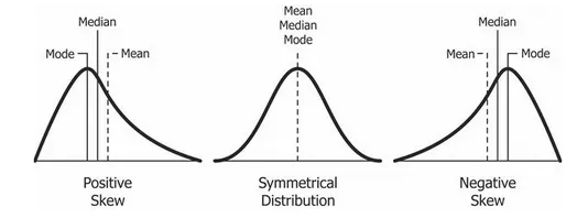
Having skewness in the curve is not a bad analysis, the skewness tells about whether the curve is symmetric or not, and it also helps us to plot the different curves in the single one, where the median and mode will be the same for different curves and thus tells us whether the curve is symmetric or not symmetric.
Mean: Average of the data sets
Median: Central value in the data sets
Mode: Repeating number in the data set
4)Evaluate the probabilities for continuous normal distribution with given mean = 680 and standard deviation = 31
a)P(X<711)
b)P(X>740)
c)P(600<x<720)
d)P(X=720)
To evaluate the probabilities for continuous and normal distribution will use 'Z- formula' and 'Z-Table'.
Z=X−μσZ=X-μσ
Where X=">`X`=Random variable
Mean(μ)=680Mean(μ)=680
S.D(σ)=31S.D(σ)=31
a) P(X<711)
Z=711−68031Z=711-68031
Z=1Z=1
P(Z<1)=0.8413P(Z<1)=0.8413 from the Z-Table.
This is the area to the left of the Z score since X is less than 711.
b) P(X>740)
Z=740−68031Z=740-68031
Z=1.94Z=1.94
P(Z>1.94)=0.9738P(Z>1.94)=0.9738
This is the area to the left of the Z score, but we need to calculate the area to the right of the Z score,
P(Z>1.94)=1−P(Z<1.94)=1−0.9732P(Z>1.94)=1-P(Z<1.94)=1-0.9732
P(Z>1.94)=0.0268P(Z>1.94)=0.0268
c)P(600<x<720)
Z=600−71131&Z=720−71131Z=600-71131&Z=720-71131
Z=−2.58&Z=1.29Z=-2.58&Z=1.29
We need to find the area for the Z score -2.58 and 1.29 subtract the values to get the probability.
P(-2.58<Z1.29) = P(Z<1.29)-P(Z<-2.58)
P(-2.58<Z1.29) = 0.9032-0.0047
P(-2.58<Z1.29) = 0.89854
d)P(X=720)
Z=1.29Z=1.29
P(Z=1.29)=0.9015P(Z=1.29)=0.9015
P(Z=1.29)=0.9015−0.9015P(Z=1.29)=0.9015-0.9015
P(Z=1.29)=0P(Z=1.29)=0
5)Explain the curve on the right side.
The given curve is the 'Normal Distribution curve' for the random variable and the percentage is the "Standard Deviations" from the mean. The distribution in the curve is perfect without any skewness. The Normal Distribution is a probability function that describes how the values of a variable are distributed.
It is a symmetric distribution where most of the observations cluster around the central peak and the probabilities for values further away from the mean taper off equally in both directions.
1σ(S.D) from the mean is around 34.1 on either side of the mean and hence the values lie b/w -34.1% and 34.1% = 68.2% of values fall in the 1 S.D region.
2σ (S.D) from the mean is taken as 34.1+34.1+13.6+13.6= 95.4% approximately the values fall in the 2 S.D from the mean.
3σ from the mean is taken as 34.1+34.1+13.6+13.6+2.1+2.1 = 99.7% approximately the values fall in the 3S.D from the mean.