Basics of ML & AL Week 2 Challenge

Calculate all 4 business moments using pen and paper for the below data set?

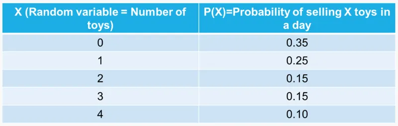
• First Business Moment - Mean

`mu = sum(X_i*P(X_i))`

`mu = (0xx0.35)+ (1xx0.25)+ (2xx0.15)+ (3xx0.15)+ (4xx0.1)`

`mu = 1.4`

• Second Business Moment - Variance

`σ^2 = sum((X_i-mu_x)^2*P(X_i))`

`=(0-1.4)^2xx0.35+(1-1.4)^2xx0.25+(2-1.4)^2xx0.15+(3-1.4)^2xx0.15+(4-1.4)^2xx0.1`

`σ^2 = 1.84`

Thus the standard deviation is 1.36. As the SD is small the data set lies near the mean.

• Third Business Moment - Skewness

`SK = sum(((X_i-mu_x)/σ)^3*P(X_i))`

`=((0-1.4)/sqrt(1.84))^3xx0.35+((1-1.4)/sqrt(1.84))^3xx0.25+((2-1.4)/sqrt(1.84))^3xx0.15+((3-1.4)/sqrt(1.84))^3xx0.15+((4-1.4)/sqrt(1.84))^3xx0.1`

`SK = 0.572139`

In statistics, skewness is a measure of the asymmetry of the probability distribution of a random variable about its mean. The skewness value can be positive or negative, or even undefined. If skewness is 0, the data are perfectly symmetrical, although it is quite unlikely for real-world data. As a general rule of thumb:

• If skewness is less than -1 or greater than 1, the distribution is highly skewed.
• If skewness is between -1 and -0.5 or between 0.5 and 1, the distribution is moderately skewed.
• If skewness is between -0.5 and 0.5, the distribution is approximately symmetric.

Thus, the given data is moderately skewed.

• Fourth Business Moment - Kurtosis

`KT = sum(((X_i-mu_x)/σ)^4*P(X_i))-3`

`=((0-1.4)/sqrt(1.84))^4xx0.35+((1-1.4)/sqrt(1.84))^4xx0.25+((2-1.4)/sqrt(1.84))^4xx0.15+((3-1.4)/sqrt(1.84))^4xx0.15+((4-1.4)/sqrt(1.84))^4xx0.1-3`

`KT = -0.95510397`

Kurtosis tells you the height and sharpness of the central peak, relative to that of a standard bell curve. The "minus 3" at the end of this formula is often explained as a correction to make the kurtosis of the normal distribution equal to zero, as the kurtosis is 3 for a normal distribution.

If the kurtosis is close to 0, then a normal distribution is often assumed. These are called mesokurtic distributions. If the kurtosis is less than zero, then the distribution is light tails and is called a platykurtic distribution. If the kurtosis is greater than zero, then the distribution has heavier tails and is called a leptokurtic distribution.

Thus, the given data has light tails and data is uniformly distributed.

What is the significance of expected value when simple mean (Sum of all observations/number of observations) is already in place?

Expected value of a random variable is a weighted(based on density function) mean. Sample mean of a random variable corresponds to average of samples.

The expected value of a discrete random, variable, X indicates the average value and is denoted as E(X). The expected value for a random variable is its mean. It is the value that you would expect to obtain if you conduct an experiment whose outcomes are represented by the random variable. It is the weignted average of all the posssible values where the probabilities of occcurane of the varibales are the weights. For a discrete random variable, the probabilities of each random variable are the weights whereas for a continuous random variable, the values of the probability density function are the weights. In probability theory the expected vavalue of random variable is the value you would expect to obtain if the random variable process was repeated for an infinite number of times and the average of those values were taken.

Basically they are same just the expected value is used to represent the expected outcome of the experiments and whose distribution is indicated by weights or probabilities.

Having skewness in the curve considered to be bad in the analysis?

In statistics, skewness is a measure of the asymmetry of the probability distribution of a random variable about its mean. The skewness value can be positive or negative, or even undefined. If skewness is 0, the data are perfectly symmetrical, although it is quite unlikely for real-world data. Skewness is neither good nor bad but helps as a tool in selecting the sample data as shown in the example below. At times when we are supposed to process the skewed data, its better to transform it.

As a general rule of thumb:

• If skewness is less than -1 or greater than 1, the distribution is highly skewed.
• If skewness is between -1 and -0.5 or between 0.5 and 1, the distribution is moderately skewed.
• If skewness is between -0.5 and 0.5, the distribution is approximately symmetric.

For normal distribution, the measures of central tendency (mean, median & mode) are equal to each other whereas for a skewed distribution, the measures are dispersed. For instance, if a distribution is positively skewed, the mean would be on the right side and for the negatively skewed data the mean would be on the left.

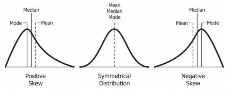
Now, we know that the skewness is the measure of asymmetry and its types are distinguished by the side on which the tail of probability distribution lies. But why is knowing the skewness of the data important?

First, linear models work on the assumption that the distribution of the independent variable and the target variable are similar. Therefore, knowing about the skewness of data helps us in creating better linear models.

Secondly, let’s take a look at the below distribution. It is the distribution of horsepower of cars:

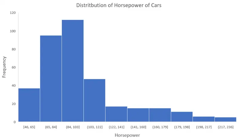
You can clearly see that the above distribution is positively skewed. Now, let’s say you want to use this as a feature for the model which will predict the mpg (miles per gallon) of a car.

Since our data is positively skewed here, it means that it has a higher number of data points having low values, i.e., cars with less horsepower. So when we train our model on this data, it will perform better at predicting the mpg of cars with lower horsepower as compared to those with higher horsepower. Also, skewness tells us about the direction of outliers. You can see that our distribution is positively skewed and most of the outliers are present on the right side of the distribution.

Evaluate the probabilities for continuous normal distribution with given mean = 680 and standard deviation = 31

Given, `mu = 680, sigma = 31`

`z= (X-mu)/sigma`

a)P(X<711)

`z=(711-680)/31`

z=1

Using the z score, lets find the probability P(Z<1) = 0.8413

Thus, P(X<711) is 0.8413.

b)P(X>740)

`z=(740-680)/31`

z = 1.9355

`P(Z>1.9355)=1-P(Z<1.9355)`

`P(Z>1.9355)=1-0.97381`

P(Z>1.9355) = 0.02619

Thus, P(Z>740) is 0.02619.

c)P(600<X<720)

P(600<X<720) = P(X<720)-P(X<600)

`Z(X=600) = (600-680)/31`

Z(@X=600) = -2.581

`Z(X=720) = (720-680)/31`

Z(@X=720) =1.29

P(@Z=-2.581) = 0.00494

P(@Z=1.29) = 0.90147

P(600<X<720) = 0.90147-0.00494 = 0.89653

Thus, P(600<X<720) is 0.89653.

d)P(X=720)

It is illogical to calculate exaclty P(X=720) as the distribution is continous and the result will lead to zero. Anyhow, the probability with continous distribution can be obtained for expected outcomes to be less than or greater than 720.

Explain the curve below?

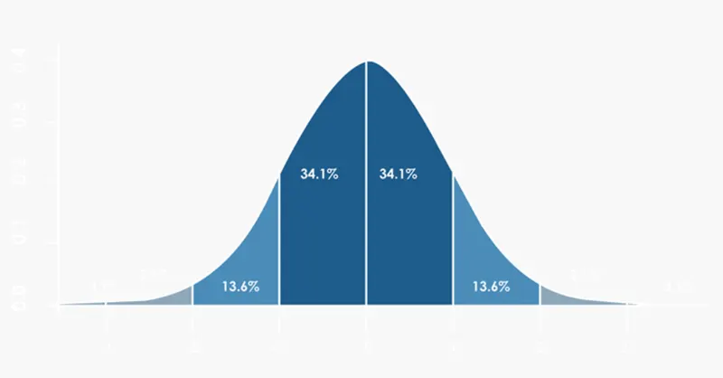
The curve above shows the standard normal distribution of data. The percentage shows the area covered under the curve (i.e., number of samples falling in the region) and the divisions are at unit standard deviation and the central line is the mean. so on the either side of mean (i.e., with in one-sigma or 1SD) 68.2% of samples reside where as with in 2 SD 95.4% samples reside and so on upon increasing the SD on either side all the samples fall under the curve making the sum equal to 1 (~100%).