Basics of ML & AL Week 2 Challenge
1.Q)
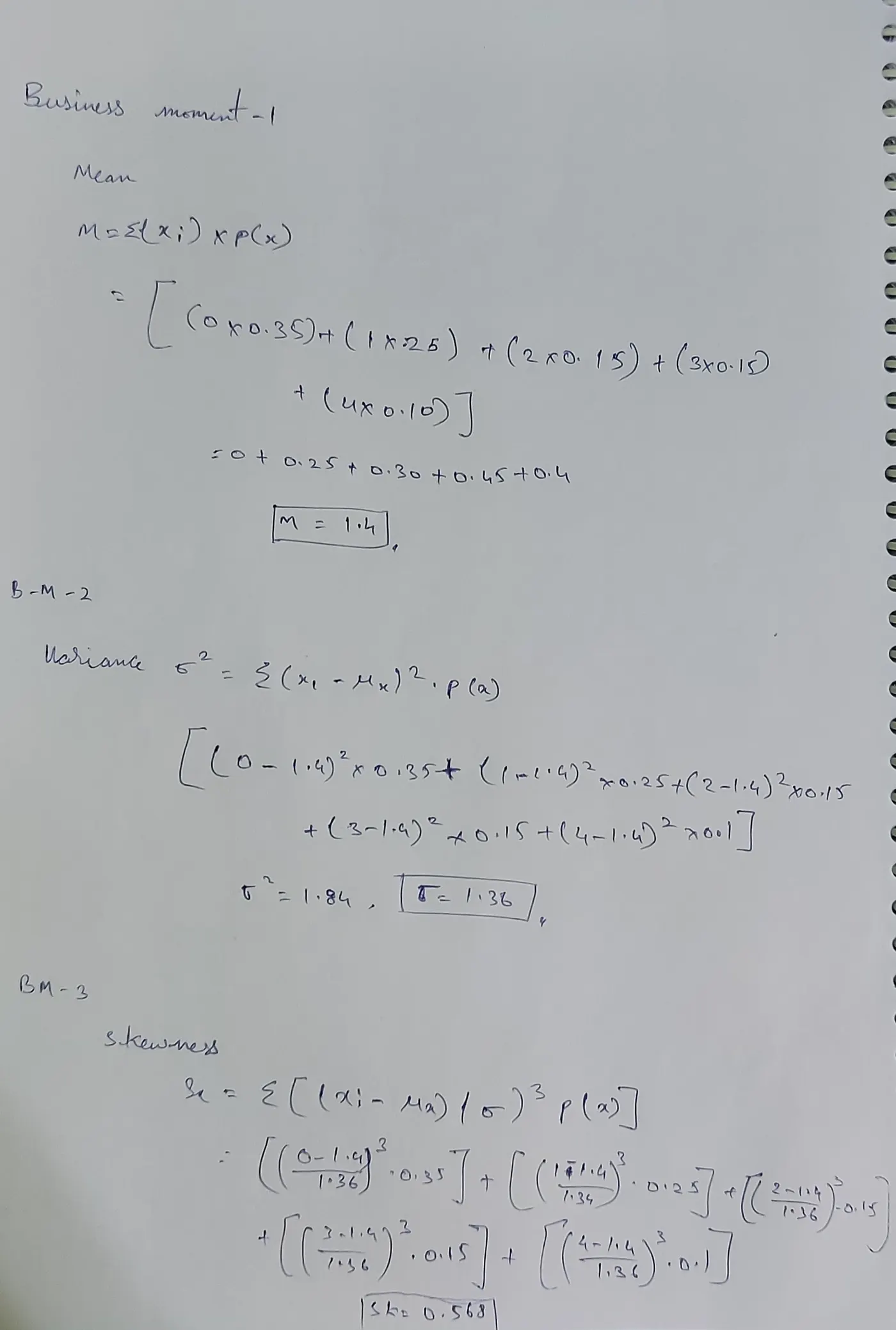
The simple mean (also known as the arithmetic mean) is a measure of central tendency that represents the middle or average value of a set of numbers. It is calculated by adding up all the values in a data set and dividing by the number of values.
Expected value, on the other hand, is a theoretical concept that represents the long-run average outcome of a random event or process. It is calculated by multiplying each possible outcome by its probability and summing up these products.
While both the simple mean and expected value provide information about the center or average of a data set, they are not necessarily equivalent. The simple mean is a descriptive statistic that summarizes the data based on its observed values, while the expected value is a probabilistic concept that reflects the theoretical distribution of outcomes.
In some cases, the expected value may differ from the simple mean due to factors such as skewness, outliers, or non-normality in the distribution.
3.Q) Skewness is not inherently good or bad in the context of data analysis. It is simply a measure of the asymmetry or lack of symmetry in a distribution. A skewed distribution can provide valuable insights into the nature of the data and the underlying processes that generated it. Many real-world phenomena exhibit skewness, such as income distributions, which are often skewed to the right (positive skewness), or error distributions in scientific experiments, which can be skewed to the left (negative skewness).
4.Q) Z-score = (X – mean) / standard deviation.
Then the z values are looked into the corresponding z-table to identify the probability less than or equal to that value.
For the given data points we have,
1. P(X<711)
The z-score of this would be = (711-680)/31 = 1.
Hence, it is one standard deviation away from the mean in the positive x axis.
In the z-table, the probability value for z = +1 is 0.8413 which is 84.13%.
2. P(X>740)
The z-score of this would be = (740-680)/31 = 1.93.
Hence, it is 1.9 times the standard deviation away from the mean in the positive x axis.
In the z-table, the probability value for z = +1.93 is 0.9732.
But it is asked for probability greater than 740. Hence, we get the value until 740 and subtract from 1.
So, the final probability value = 1 - 0.9732 = 0.0268 or 2.68%.
3. P(600
In this case, we need to find the value of probability at X<720 and X<600 and subtract both values.
When X = 720, z = 1.29 and probability value is 0.9015
When X = 600, z = -2.58 and probability value is 0.00494
Final probability value = 0.9015 – 0.00494 = 0.89656 or 89.656%.
4. P(X=720)
The approximate value is: P(X=720) = N(1.433,1)=0.9288 or 92%
5.Q)
Here, the mean of this observation data is always 0 and the standard deviation is 1.
It gives us the percentage of data falling under every 1, 2 and 3 standard deviation from the mean value. In this figure, 68.2% of data falls from z values -1 to +1, 95.4% from -2 to +2 and 99.6% from -3 to +3.
An example application of this graph would be the results of IQ test of people living in a city.
It can be noted that not everyone would have gotten the highest IQ or the lowest. Most of the range would be around the mean value which is depicted by this graph. Another example would be marks obtained in a test. It can be observed that people who score centum and people who scored a zero would be very less. More students’ marks would be around the average class mark.