Basics of ML & AL Week 2 Challenge
Note: I do Q1 in Excel, but answers vary from my calculation so I didn't attached it.
1)Calculate all 4 business moments using pen and paper for the below data set
1) mean µ= ∑(x1) * p(x)
= 0*0.35+1*0.25+ 2*0.15 + 3*0.15 + 4*0.10
= 0 + 0.25 + 0.3 +0.45 +0.4
= 1.4
2) Second business movement
Variance σ2 = ∑(x1-µx)^2 *P(x)
σ2 = (0-1.4)^2 *0.35 + (1-1.4)^2 *0.25 + (2-1.4)^2 *0.15 + (3-1.4)^2 *0.15 + (4-1.4)^2 *0.10
σ2 = 0.686+0.04+0.054+0.384+0.676
σ2 = 1.84
3) Third Business movement
σ = 1.356
Skewness (SK) =∑((xi-µx)/σ)^3* P(x)
= ((0-1.4)/1.356)^3 *0.35 + ((1-1.4)/1.356)^3 *0.25 + ((2-1.4)/1.356)^3 *0.15 + ((3-1.4)/1.356)^3*0.15 + ((4-1.4)/1.356)^3 *0.10
= -0.3851+ (-0.00641) + 0.0129 + 0.246 + 0.704
= 0.57139
4) Forth Business Movement
Kurtosis (Kt) =∑((xi-µx)/σ)^4 *p(x) -3
= (((0-1.4)/1.356)^4*0.35 + ((1-1.4)/1.356)^4*0.25+ ((2-1.4)/1.356)^4*0.15+ ((3-1.4)/1.356)^4*0.15 + ((4-1.4)/1.356)^4*0.10)-3
= (0.3976 + 0.00189 + 0.00574 + 0.2907 + 1.3516)-3
= -0.97665
= -0.98
2)What is the significance of expected value when simple mean (Sum of all observations/number of observations) is already in place
The application of simple mean and expected value are dependent on the nature of the case study. In smaller case studies where the random variable outcomes can be measured as the frequency of occurrences or each observation in the sample can be noted, the sample mean is calculated sum of all observations/number of observations`
However, in a case of an infinite number of observations, it is very difficult to note every outcome of the given dataset. In such cases, the probability of each outcome is determined using a sample study and using this probability the expected value is determined using. The expected values reduce the analysis expenditure and serve the purpose of measuring the central tendency of the data set.
Mean or expected value, μ=∑x.P(x)">μ=∑x.P(x)μ=∑x.P(x)
The expected value is an anticipated value for investment at some point in the future. in statistics and probability analysis, the expected value is calculated by multiplying each of the possible outcomes by the likelihood each outcome will occur and then summing all of those values. by calculating expected values, investors can choose the scenario most likely to give the desired outcome.
The expected value is calculated as follows for e.g the player plays occur as the probability of occurrence is given by the probability that they play zero days is 0.2 the probability that they play one day is 0.5 and the probability that they play two days is 0.3.
Here the days are random variables 0 days, 1 day, and 2 days the occurrence of appearance is 0.2,0.5, and 0.3.multiplying both will give 0,0.5 and 0.6, and summing up will give expected values as 1.1. The sample mean varies with the frequency of appearance in the occurrence of the variable hence the sample varies with the value.
3)Having skewness in the curve considered to be bad in the analysis?
Skewness refers to a distortion or asymmetric that deviates from the symmetrical bell curve or normal distribution in a set of data. if the curve is shifted to the left or the right it is said to be skewed. Skewness can be quantified as a representation of the extent to which a given distribution varies from a normal distribution. A normal distribution has a skew of zero.
Having skewness in the curve is not a bad analysis the skewness tells about whether the curve is symmetric or not and it also helps us to plot the different curves in the single one where the median and mode will be the same for different curves and thus tells us whether the curve is symmetric or not symmetric. Mean - Average of data sets, Median - Central value in the data set, Mode- Repeating number in the data set. Linear models work on the assumption that the distribution of the independent variable and the target variable are similar. Therefore knowing about the skewness of data helps us in creating better linear models.
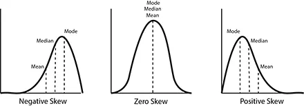
A positive Skewed distribution has the tail on its right side. The value of skewness for a positively skewed distribution is greater than zero. As you might have already understood by looking at the figure the value of the mean is the greatest one followed by the median and then by mode. Well, The answer to that is the skewness of the distribution is on the right it causes the mean to be greater than the median and eventually move to the right. Also, the mode occurs at the highest frequency of the distribution which is on the left side of the median.therefore mode<Median< mean.
A negatively skewed distribution has the tail on its left side. The value of skewness for a negatively skewed distribution is less than zero. From the above, we can understand that skewness doesn`t have any bad effect on analysis rather it helps us identify certain characteristics of the data set just by looking at the graph. This proves to be very effective in data analysis and has no bad effects associated with it.
The general skewness is neither good nor bad without knowing the application of the data or the purpose for what it was obtained. Different applications have different meanings for skewed or non-skewed data. A distribution can have a positive skew no skew or a negative skew or even be undefined.
4)Evaluate the probabilities for continuous normal distribution with given mean = 680 and standard deviation = 31
a)P(X<711)
b)P(X>740)
c)P(600<x<720)
d)P(X=720)
me
z= X - Mean / Standard Deviation
a) P(X<711)
= 711- 680/31
= 1
a) P(X>740)
= 740 - 680 /31
= 1.935
c)P(600<x<720)
1) = 600 -680 /31
= -2.58
2) =720-680 / 31
= 1.29
P(-2.58 <Z< 1.29) = P(Z<1.29) - P(Z<-2.58)
= 0.9015 -0.0049
= 0.8966
= 89.66%
d)P(X=720)
= 720 -680/ 31
= 1.29
find the z probability
P(z=1.29) = P(1.29<Z<Z1.29)
= 0.9015-0.9015
= 0
5) Explain the curve on the right side
The graph given below shows the normal distribution of the data points by plotting the z-values with their corresponding probability values.
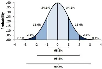
Here, the mean of this observation data is always 0 and the standard deviation is 1.
It gives us the percentage of data falling under every 1, 2, and 3 standard deviation from the mean value.
In this figure, 68.2% of data fall from z values -1 to +1, 95.4% from -2 to +2, and 99.6% from -3 to +3.
An example application of this graph would be the results of IQ tests of people living in a city.
It can be noted that not everyone would have gotten the highest IQ or the lowest. Most of the range would be around the mean value which is depicted by this graph. Another example would be marks obtained in a test. It can be observed that people who score a centum and people who scored a zero would be very less. More students’ marks would be around the average class mark.