Assignment 7-Side Pole Crash Simulation Challenge

1. AIM:

The main aim is to perform side pole crash analysis in the neon model with the recommended parameters and output requests.

• Neon side crash-BIW

• Check the unit system and either follow [Mg mm s] or [Kg mm ms].
• Check an appropriate interface, friction 0.2 and recommended parameters.
• Make sure of no penetration and intersections.
• Create a rigid pole with a friction of 0.1 as per the FMVSS 214 standards.
• Compare the model weight with the reference model and use added masses to reach the target weight of 700kg while getting CG about the required range.
• Initial velocity - 20mph, as per the standards.
• Use a model checker to ensure good quality.
• Timestep:0.5 to 0.1 microseconds.
• Run 80ms.

• Output requests
• Sectional force in the cross member.
• Intrusion at B pillar, hinge pillar and fuel tank region.
• Provide recommendations on what can help to reduce Fuel tank intrusion.
• Peak velocity of an inner node of the door.

2. Procedure:

• Step – 01 Intersection and penetration checking: -

1. Open the hyper mesh with user profile as RADIOSS.
2. Import the starter file in Radiosss.

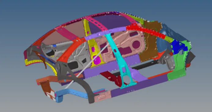
Fig 1: Given Side pole crash vehicle component

• Check the unit system under begin card. This model has unit system of [Kg mm ms].

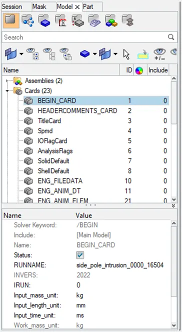
Fig 2: Unit system in begin card

1. Go to tools – Penetration check – select all the components – check.

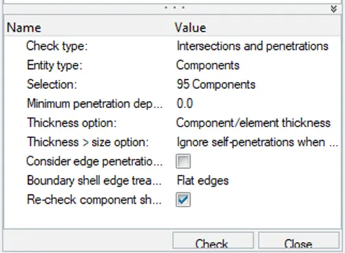
Fig 3: Penetration check

1. There are no penetration or intersection errors found.

• Step – 02 Balancing COG: -

1. The model does not have exact weight of vehicle. So additional mass should be added to model.
2. The targeted weight is given 700kg where the actual mass before adding external weight is 166kg.

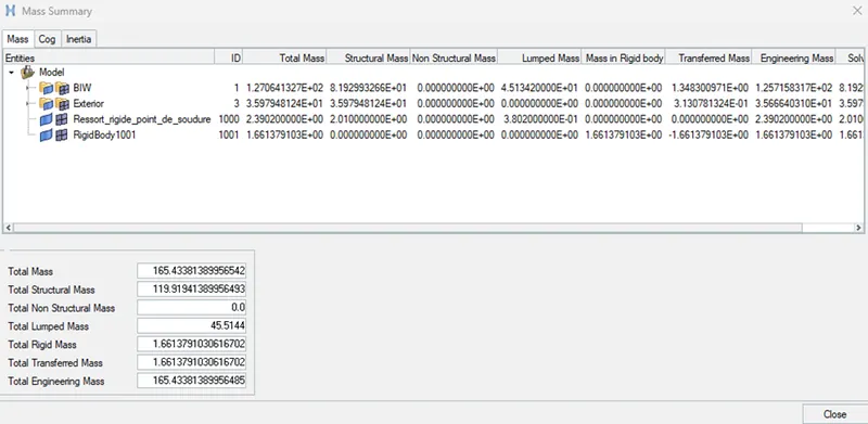
Fig 4: Before mass added to the model

1. Right click on solver menu to create ADMAS and select the mass type & nodes.
2. Add mass according to the needs till the point reaches the centre and till the mass attains the target value.

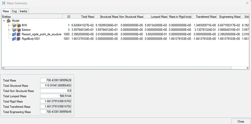
Fig 5: After mass added to the model

• Step – 03 Creating contact surfaces: -

1. Right click on Solver menu – create interface – Type 07.
2. Before creating contact surface make sure delete the previous interfaces.
3. Select all the components and enter the Istf, Igap, Idel and other values.

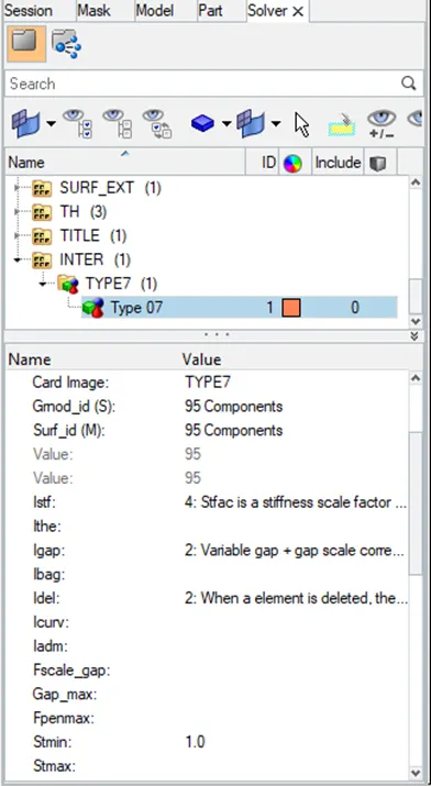
Fig 6: Contact surface created

• Step – 04 Rigid wall: -

1. Right click on Solver – Rwall – CYL – Geometry type as Cylinder.
2. Enter the co-ordinates, Friction, Diameter & DSearch.

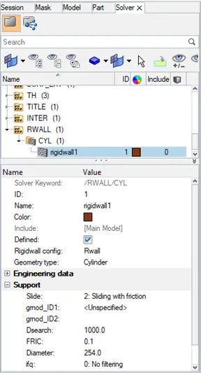
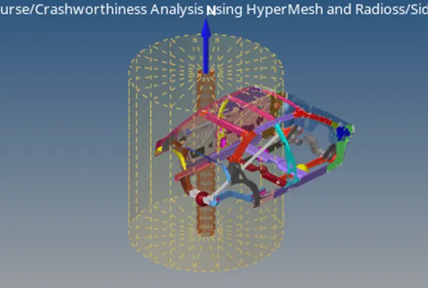
Fig 7: Cylindrical Rigid wall Created

1. The normal direction to the pole in Z-axis and diameter of the pole to be 254 mm.
2. The FRIC value will be 0.1 and Dsearch value will be 1000.

• Step – 05 Initial Velocity: -

1. In this simulation the initial velocity given to the model is 35Mph or 15.6464 mm/ms.
2. Go to Load case – initial velocity – set the values in Y direction – select all the nodes.

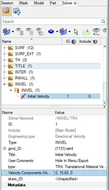
Fig 8: Initial Velocity Created

• Step – 06 Section Creation: -

1. Before creating cross section, create moving frame on nodes also called local axis.
2. Right click on solver browser, create – Frame – MOV – Select nodes – create.
3. Once frame created. Right click on solver browser – create – sect – SECT – specify the frame ID & nodes.
4. Right click to create grshel_id and enter Delta & Alpha values.
5. Create cross section for both the cross members.

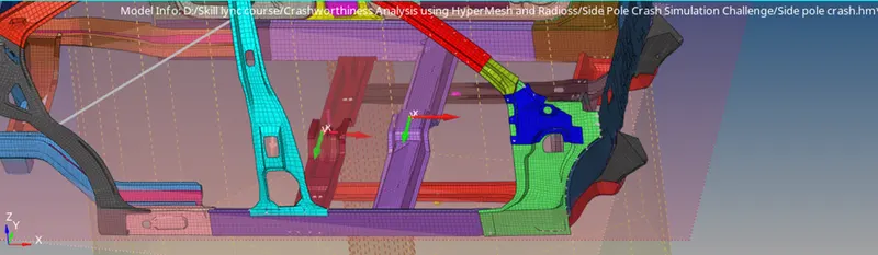
Fig 9: Cross section Created

• Step – 07 Requesting for output files: -

1. Right click on model browser – create new output blocks – select the entity ID’s (Cross sections) – create.

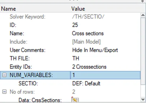
Fig 10: Output blocks Created

1. To find peak velocity of inner node of door.
2. Go to solver browser – Right click – SKEW – MOV.
3. Select the nodes and create.
4. To measure the intrusions at B-Pillar, hinge pillar & fuel tank.
5. Create spring on both side of B-Pillar, hinge pillar & fuel tank.
6. Go to 1D – springs – spring2 – select the nodes.
7. Now create property card for springs and assign spring elements.
8. Go to model browser – create - property – rename as intrusion springs.
9. Select the card image as P4 springs and enter mass & stiffness values.

• Step – 08 Requesting for output for springs: -

1. Go to solver browser – create – TH – Springs.
2. Select the elements and follow the same other two elements.

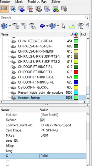
Fig 11: Spring Property card Created

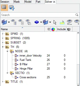
Fig 12: TH files Created

• Step – 09 Time step & Run time: -

1. To check the parameters in hypermesh, Go to model browser – cards.
2. Change the TSCALE (0.67) & Tmin (0.001) values in ENG_DT_NODA.
3. Change the TSCALE (0.9) & Tmin (0.0001) values in ENG_DT_BRICK.
4. Change the TSCALE (0.67) & Tmin (0.0005) values in ENG_DT_INTER.
5. Open ENG_RUN card and input run time in Tstopas 80 ms.
6. Go to ENG_ANIM_DTcard enter T freq as 5.

• Step – 09 Run model checker to ensure good quality: -

1. Go to tools – Model checker – Radioss block.
2. Click the Run check command and errors are indicated as RED colour.
3. After running the checks, we get zero errors only warning is shown we can ignore these warnings and move further.

.

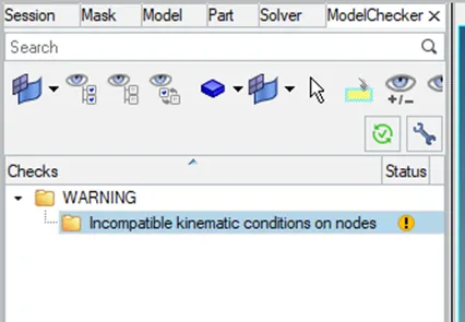
Fig 13: Model checked

• Processor: -

1. Now run the simulation. Go to Radioss in analysis.
2. Specify the path to save the file and type ‘-nt 4’ In option.
3. Click Radioss and run the simulation.

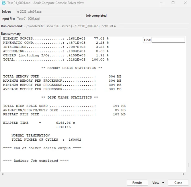
Fig 14: Analysis Done

1. First check for Energy & mass error.
2. Open Engine.out file of the model and check the energy & mass error.

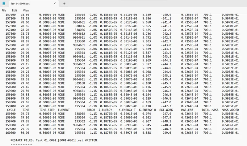
Fig 15: Energy & Mass Error

1. The Energy errorwhich is -1.1% and Mass error which is very negligible. This shows that the energy error and mass error are within acceptable range.
2. Total number of cycles used id 160002 and total run time of simulation is 6165.96s.
3. Open hyperview to view animation and contour plot.
4. Select the Displacement & von misses in result type and simple in averaging method.

VON MISES STRESS CONTOUR PLOT: -

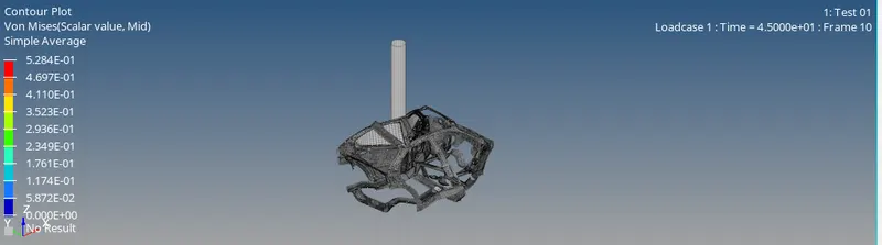
1. After generating the simulation, generate the plots using Hypergraph.
2. In Hypergraph, import the T01 file to plot the graph.

GLOBAL VARIABLES ENERGIES PLOT: -

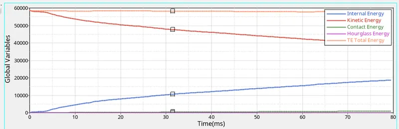
1. From the above plot, we can see that there is high amount of Kinetic energy at the start of the simulation but as the simulation progresses, the kinetic energy in the vehicle decreases and gets converted into internal energy, so the internal energy increases in the same proportion.
2. Thus, the total energy in the system is almost constant at 85000 kg*mm2/ms2and due to some energy loss, which we can see in energy error, there is some decrease in total energy.
3. We can also see some amount of contact energy in the model as we have defined the value of friction in Type 7 interface due to which contact energy is generated.

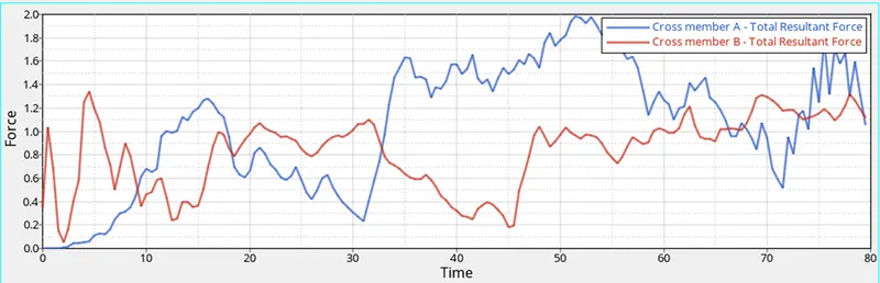
CROSS SECTIONAL FORCES ACTING IN CROSS MEMBER: -

INTRUSION: -

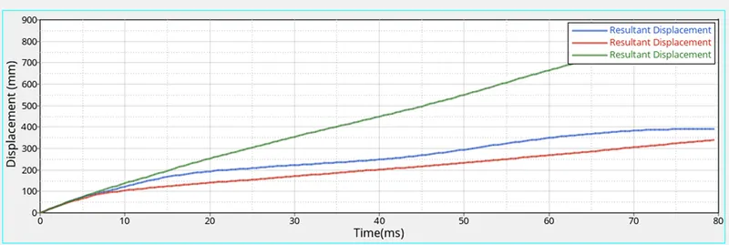
Blue line – Intrusion node at fuel tank

Red line – Intrusion node at B-Pillar

Green line – Intrusion node at Hinge Pillar

PEAK VELOCITY OF INNER NODE OF DOOR: -

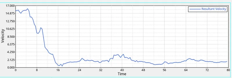
This plot helps to understand, with how much the actual inner side of the door moves in the direction of the Driver during the pole impact. The peak Velocity measure at the inner door point is 15.84mm/ms till 8 ms. after that, the speed is starting to reduce to a great extent.

Conclusion:

Thus, the model was simulated for a side pole crash test and the results were discussed. From the output file the energy error and mass error are in an acceptable range so I can conclude that the simulation is pretty stable. Cross-members A and B are playing important role in the Impact force absorption. So, improving the cross-member material or adding some extra support element near the cross member can improve their performance, also for the Fuel tank side as we discuss earlier need some reinforcement. We can also work on the B-pillar property improvement as it's the closest part which is comes in the contact with the force during the side crash.