AIM:
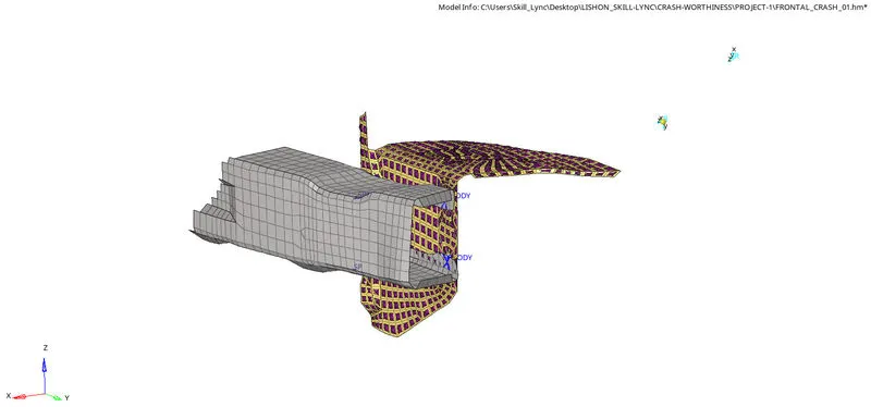
To analyse and simulate the frontal crash of a BIW car and thereafter observe the resultant output request and energy differences across the model.
OBJECTIVE:
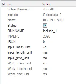
- Check unit system, which has to be followed in [Kg mm ms].
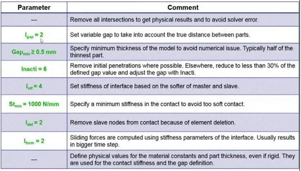
- Create appropriate interface with friction 0.2 and recommended parameters (TYPE 7)
- Make sure of no penetrations, intersection and flying parts exist in the model.
- Check all rigid bodies in the model and rectify if there are any issues.
- Create rigid plane wall with friction 0.1.
- Compare the model and use added masses to reach target weight 700kg while getting Centre of Gravity about the required range.
- Initial velocity of the car has to be 35 mph.
- Use model checker to check for errors in the model to ensure good quality
- Time-step has to be in between 0.5 to 0.1 microseconds.
- Run the simulation for 80 ms.
In the output request check for:
- Sectional force in the rails at location of indicated node- 174247.
- Axial force or normal force received on the rails from bumper.
- Shotgun cross sectional forces.
- A pillar cross section.
- Acceleration curve received on the accelerometer at base of B pillar (on B pillar rocker).
- Intrusions on the dash wall on nodes 66695 and 66244.
INTRODUCTION:
The simulation of vehicle crashes by using computer softwares has become an indispensible tool for shortening automobile development time and lowering costs. It also has huge impact on the crashworthiness of an automobile. This work reports on the simulated frontal crash test of an automobile. The objective of this work is to simulate a frontal impact crash of an automobile and validate the results. Computer models were used to test the crash characteristics of the vehicle in the crash. The software used for the simulation is HYPERMESH AND HYPERCRASH. It is widely used by the automotive industry to analyze vehicle designs. It accurately predicts a car's behavior in a collision.
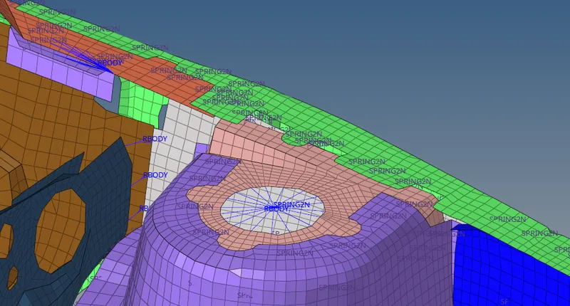
Crash-Test:
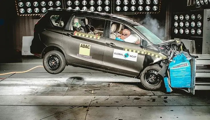
A crash-test is a form of destructive testing usually performed in order to ensure safe design standards in crashworthiness and crash compatibility for automobiles or related components. To test the cars safety performance under various conditions and during varied types of crashes, vehicle manufacturers crash test their cars from different angles, different sides and with different objects, including other vehicles.The main purpose of a crash analysis is to see how the car will behave in frontal or/and sideways collisions. Car body light weighting and crashworthiness are two important aspects which are considered while designing any vehicle. The chassis frame forms the backbone of the vehicle. Its main function is to carry maximum load for all designe operating condition. This is a part of designing cycle which can reduce the need for costly destructive testing program. This method has a great scope in all automobile industry as it reduces the cost of actual crash testing of the vehicle. Due to participation of various companies the customers have a variety of vehicles to choose. Hence, all the companies are adopting this method of simulation to minimize the weight as well as to make the vehicle safe.
PROCEDURE:
INITIAL SETUP:
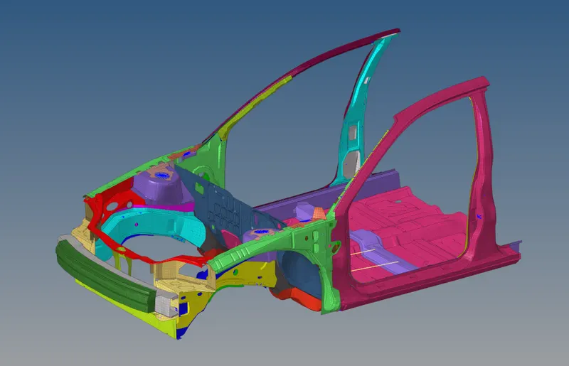
1. Select the starter file from the file location with name neon_front_0000 and import the model in the Hypermesh software. Check if the User profile has been changed to Radioss.
2. Similarly open the Hypercrash software from the Hypermesh window by going to the application option. Change the unit system to (Kn,mm,ms,kg) and Run, which will succesfully open the Hypercrash software.
3. Drag the same file into the Hypercrash panel so that the model can be opened easily.
4. First, check for the unit system as given by default in the HM software. This can be checked by going to the BEGIN_CARD in the Engine card.
5. Since all the simulations are done in the hypermesh, so whatever setup which has to be done in Hypercrash should be done first, so that exporting has to be done only once, which would save the overall time.
6. Next will be the mass addition inorder to attain the required mass and bring CG to the correct position.
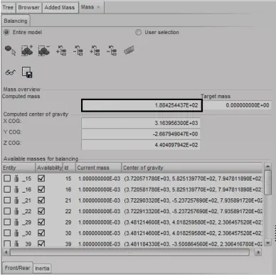
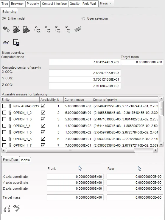
7. Check the current mass of the model by going to Mass-> Balancing, under which the mass overview computed mass tab will show the overall mass of the body. The COG of the model can be visually inspected by clicking on the Show COG point avilable in the same tab.
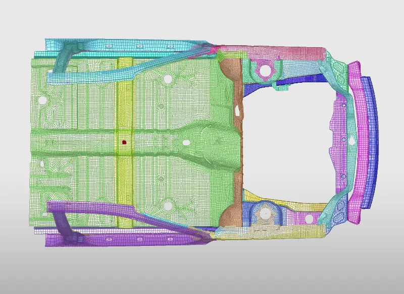
8. The idea or objective is to bring the COG point in between the centre point of driver and passenger seat with the total mass resulting in a value equal to 700kg. Both of them have to be done simulataneously which means when the mass becomes 700kg the COG point should lie on the above mentioned position.
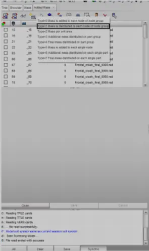
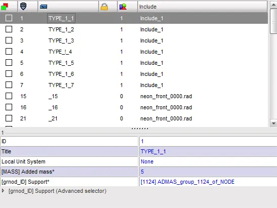
9. The mass can be added by going to LoadCase-> Addedmass and create a TYPE 1 Mass where mass is added to each node of the node group. Depending upon the position of the COG, the mass can be added to each positions in the model.
10. After selecting the TYPE 1 mass, a drop up box will come where in the option of (grnodeid)support, select the nodes where the mass has to be added and in the Added mass option specify how much unit of mass which has to be added.
11. The total mass has reached to a value of 700kg and the COG of the model has been made to the required position in between the front seats which is shown below:
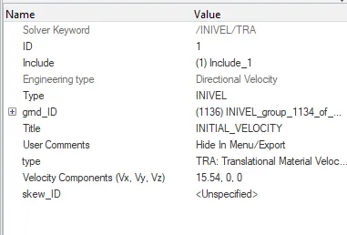
11. Next is the initial velocity which has to be added to the car inorder to hit the barrier with a velocity of 35 mph or 15.64 mm/ms which is the same value followed in the crash test in industries.
12. This can be done in the HC software by going to Loadcase-> Initial velocity, where a new tab box will be opened.
13. The Type has to be given as 0:translational. Since the carcrashes in the positive X direction, the velocity X has to be given as 15.64 and in the [Gnod_ID]Support, select all the nodes of the car component.
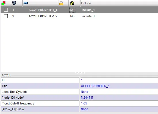
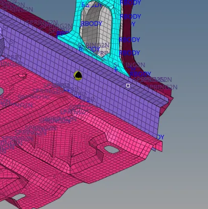
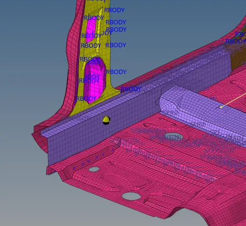
14. Next is the Accelerometer which has to be given on the base of B-pillar (on B-pillar rocker). Accelerometer entities are defined by a node and a local coordinate system of type SKEW. This coordinate system is not mandatory. If it is not defined, accelerations are measured in the global coordinate system, otherwise, in the defined local coordinate system.
15. This can be opened by going to the Data history-> Accelerometer, where in the tab opened, select the node and the Fcut[Cut-off frequency] has to be given a value of 1.65. The next Accelerometer has to be gievn exactly oppposite to the other node of the
B-pillar rocker. Follow the same procedures as that of the first Acccel.
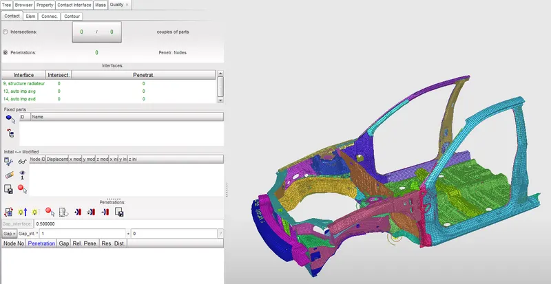
16. Next is to check for penetrations and intersection, which can also be done in the HC, Goto Quality -> Check all solver contact interface. Here there are no penetrations and intersections formed in the model. If there are any, click on Depenetrate Auto option which will remove most of them automatically. The rest can be removed using the Translate tool available in the Tool panel.
17. As all the setup in the Hypercrash has been finished, export the model from the HC and import in the Hypermesh software.
18. Once it is done, next step is to create appropriate interface for the car which is the self-impact for the car. Check whether there are any default interfaces, if any delete all the ineterfaces from the Groups in the Model browser.
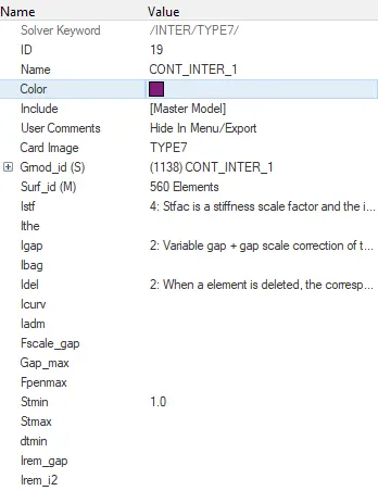
19. Now a new Interface has to be devoloped by selecting the Solver-> Create-> Inter-> Type7.
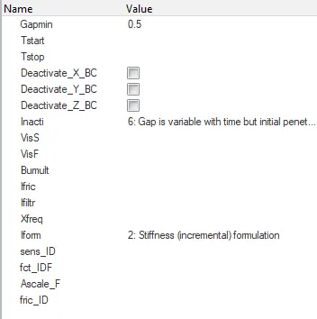
20. In the interface formed, select the recomended propertes which are shown below:
21. Ensure that the friction value is given as 0.2 along with the recommended property values.
22. Next is to check the rigid body connections in the model and if there are any, give proper connections. Since this model has been given with all proper rigid connections, so no other extra connections has to be given. An example of rigid is shown below:
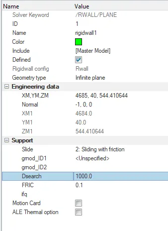
23. Next is to create a plane rigid wall, for that goto Solver->Create->RWall->Plane. Thus an Rwall folder will be created. In the dropdown box input the values, starting with the Engineering data where we have to give the co-ordinate values for where we have to form the rigid wall.
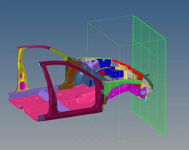
24. Inorder to get the co-ordinates, create two temporary nodes on the centre part of the bumber and translate those two nodes to a sufficient distance so that a minimum gap is given in between the car and the Rwall. Use these points for the co-ordinates as well as for the vector directions. The normal has to given in X axis but opposite to the direction (ie. direction towards the car from the RWall). In the support option give the slide property as 2:sliding with friction with friction value as 0.1 as given and the Dsearch value in between 1000-2000.
The devoloped Rwall across the car is shown below:
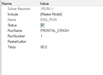
25. Then give the runtime for the simulation as 80ms which is the Tstop. Inorder to change the run time goto Model->Cards->Eng_run->T_stop, where you can change the runtime as required.
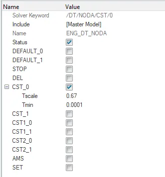
26. Next as per the given question the timestep of this model has to be in between 0.5-0.1 microseconds. When converted the value we input is 0.0001ms. Inorder to change this value goto Model->Cards->Eng_DT_noda-> check CST_0 where two suboptions will be formed->change Tscale as 0.67 and Tmin as 0.0001
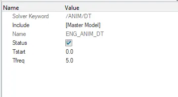
27. In Eng_Anim_DT the time frequency has to be 5.
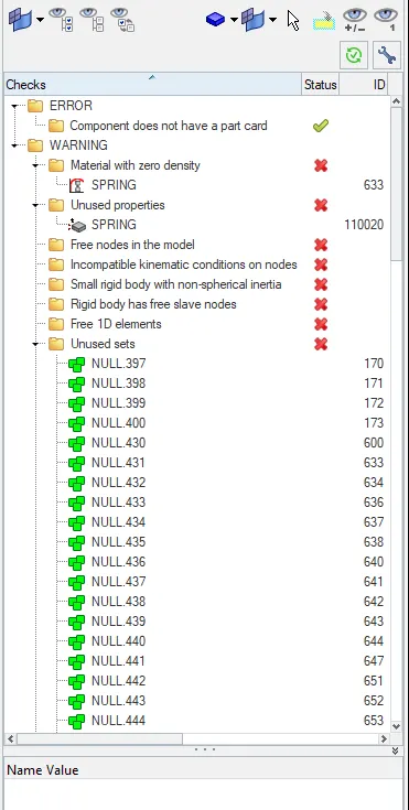
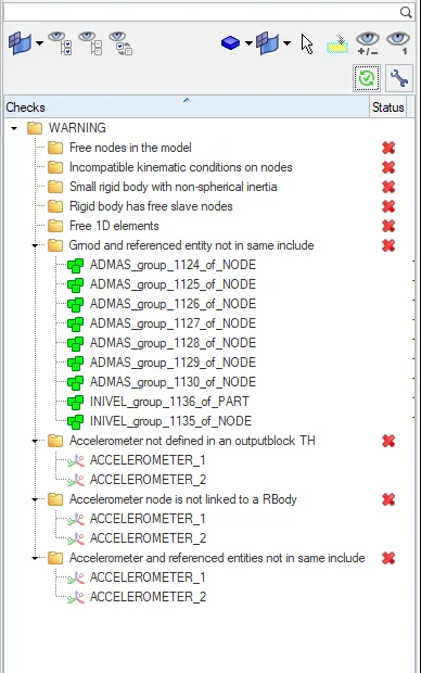
28. After completing the initial setup, to check whether the model is free with errors and to know whether it is good, the Hypermesh gives as an option called Model Checker, by which after running it, tells us whether there are any errors in the model or not.
29. Inorder to open the model checker, goto Tools-> Modelchecker->Radioss and another browser will be opened where select the option to run and if any error shows, rectify it. The below image shows that the model is free from errors. The warnings formed can
be leaved as such as it wont affect the model during the time of simulation.
OUTPUT REQUEST:
Sectional Force:
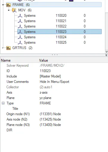
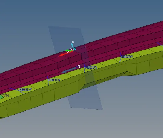
Sectional forces are created in the components inorder to get the forces acting along a particular cross sectional area. As given the sectional forces has to be created in Rail, Shotgun and A-pillar. Inorder to create a section, first Frame has to be craeated.Frames are type of local co-ordinate system where its quantities are defined to follow its own origin. First create the frame and section in the Rail.
1. Inorder to create the Mov frame goto Solver->Frame->MOV. In the panel opened, select the option of Create by node reference.
2. In the origin node option, select the node which has to be selected as the origin for the co-ordinates. Then select the next node adjacent to the other node, inorder to devolop the Z-axis, which has to be normal to the direction of force or to the Rwall. At last, select the XY-plane by clicking on the next node clockwise to it.
3. This will create a MOV Frame at that particular region.
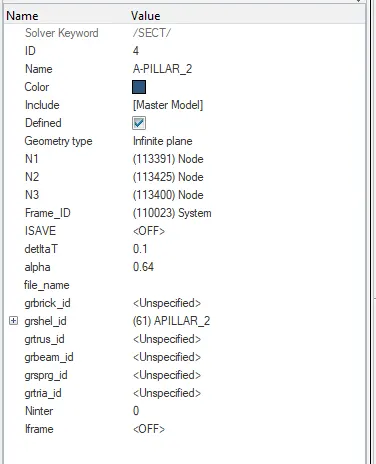
4. Next create a section in the same place. Inorder to create the section goto Solver->Sect->SECT. This will create a SECT file in the solver browser.
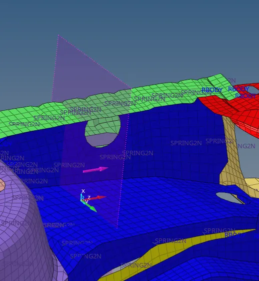
5. In the tab opened, select the three nodes N1,N2,N3 for creating the section. These three nodes have to be same as that of the earlier nodes selected for the same in the same order. the Frame_ID has to be assigned in this section. The constant parameters of deltat and alpha has to be given values of 0.1 and 0.67 respectivily. Last, in the grshel_id, select the elements in a way around the frame such that a sectional crosssection has to formed. For that select atleast two rows left and right from the origin co-ordinates.
6. After creating the section, check whether the direction of the section formed is normal to the Rwall.
7. Similarly create the cross-sections for the other rail where the node has to be selected exactly opposite to the node selected. Likewise two sections in shotgun as well as A-pillar has to be created.
AXIAL FORCE RECEIVED ON RAILS FROM BUMBER:
The Axial force is the force received along the line of impact{ie. X-axis}. Inorder to give the output request for Axial force, a contact interface has to be created with TYPE 7 with the recommended properties. So two interfaces has to be created on either sides of the bumber so that it can be analysed easily.
1. Inorder to create the interface goto Solver->Inter-> Type 7. Thus an inter file will be created. Name it as cont_iner_right.
2. Here we have to assign the master and slave node. The component under study is usually the master and the component which is used as the barrie is the master. In this case the bumber is considered as the slave while the rail is the master.
3. In the Surf_id select the component rail and in the grnod_id select the nodes of bumber portion which will come in contact with the rail.
4. A shown earlier all the recommended properties of Type 7 has to be assigned.
5. Similarly following the same above steps, create a interface on the left side of the bumber-rail portion.
INTRUTIONS ON THE DASH WALL:
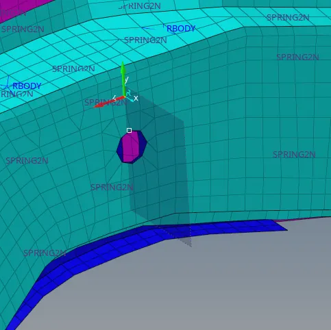
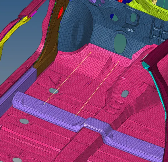
Intrusions are generated inorder to understand the change of displacement happened during the time of deformation. This can be achieved by creating a spring element using the two node option. As given two spring elements have to created with reference of nodes 66695 and 66244. So two temporary nodes have to be created exactly opposite to these specified nodes using the translate option.
1. Inorder to create the spring, goto 1D panel and select Rigids. Select the two nodes where to generate the spring. Similarly the other spring also has to be created. In the pop-up box, change the card image to Part.
2. Create a property for the spring and assign the card image to P4_SPRING and the mass value to 0.001 and the stiffness (k1) value to 0.001
TIME HISTORY FILES:
The time history files have to be given to all the output request commands where the graph has to be plotted in the Hypergraph 2D. I this simulation, we add the INTER, ACCEL, SPRING and SECTIO for the contact interfaces, accelerometer, Intrution springs and cross-sectional forces respectivily. Inorder to create the TH file
1. Goto the Solver->TH-> select whichever files needed.
2. For the INTER file created, the Entity ID has to be assigned. Select the number of variables as required and in the Date: INTER, select the parameters needed for plotting the graph.
ENGINE CARDS:
Check that all Engine cards have been properly created with the correct timestep as wel as the runtime which will totally affect the total time taken for the simulation.
1. Create the Eng_DT file and give the Tmin value.
2. In Eng_Run, give the runtime as 80ms.
3. IN eng_anim_DT, give the Tfreq as 5
MODEL CHECKER:
As explained earlier, the model checker has to be runned again to check whether the model is free from errors.
Also delete all the empty as well as Unused files from the model. Goto Tools-> where we will get the option for UNused and Empty. Check it and delete all the files in that inorder to avoid warnings.
SIMULATION RESULTS WITH GRAPH PLOT AND ANIMATION RESULT:
After all the initial setup and output request has been assigned for the given model, next the main step is to run the simulation. It may take upto 5-6 hrs depending upon the configuration and speed of the computer.
To run the simulation, following are the steps to be followed:
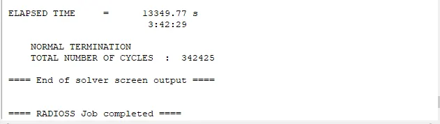
1. Run the simulation by going to the Radioss in the Analysis panel. Browse the location where the simulation file is saved. Check the runned simulation ends with Normal Termination.
2. Check the export option have been turned to All, Run option as analysis and the run number as 1 and check connectivity is turned on. In the option type -nt 4 has to be written to increase the speed of the simulation by four times. Click on radioss.
3. At this time, the simulation starts to run and it may take a while longer, depending upon the model.
4. Change the hypermesh panel to Hyperview panel and browse the animation file from the previous saved simulation result folder. The Anim file will be in .h3d format. Click apply.
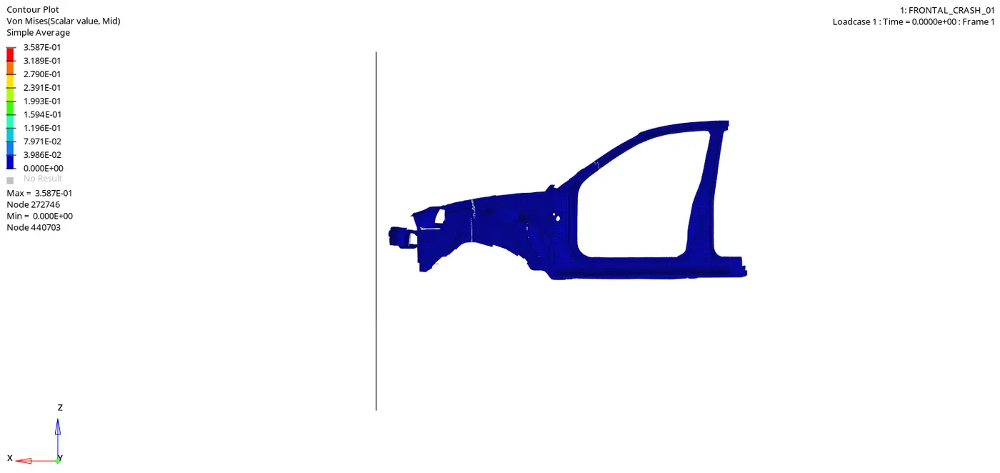
5. The animation file with the vehicle crashing the rigidwall be be created.
6. Now split the window and open the Hypergraph 2D panel.
7. In the same simulation file check for T01 file and upload it in the Hypergraph.
8. Below that we can see the X Type and Y Type which is nothing but the X component and Y component.
9. On X axis, select the time as the constraint while in the Y axis, it is subdivided into three:
- Y Type
- Y Request
- Y Component
ENERGY PLOT:
This includes all the energies including KE, IE, CE, HE acting in the model during the time of deformation.
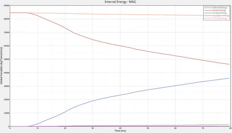
- Kinetic Energy: The kinetic energy of this model starts with a very high value from the initial stage and then gradually decreases.This is because at the initial stage of deformation happens with very high velocity and with applied mass of the body.But with time, when the force moves along the surface, some energy will get disscipated along the path.So there will be slow decrement in the value of kinetic energy.
- Internal energy: It is the sum of kinetic energy and potential energy.when t=0 , the internal energy is zero till the time of collision, as there where no deformation happening currently.But when the deformation starts, frictional force is devoloped along with some heat dessipation.With the intensity of deformation, the energy will be absorbed and the internal energy will be increased.
- Hourglass energy: The summation of displacements and force sometimes provide zero strain and stress values and then the element fails to calculate the stiffness values.When it fails in such a way, it will result in some weird deformation and results in the formation of hourglass energy.Since the Ishell is given as QEPH 24 is applied in the property tab as default, the hourglass energy is reduced to zero with the physical stabilization happening in the material level itself.
- Contact energy:This type of energy is formed when one element comes in contact with the other or neighbouring elements.The opposing force created by this element forms the contact energy.At the first stages of deformation, the contact energy goes constantly without any increase. But at the end of the simulation, with the high deformation or crushing happens, the contact energy will be devoloped and increases slightly. But in the above graph with all energy plotted in a single graph, the contact energy tends to form negligible.
- Total energy: The total energy of the system is the summation of all the energies happening with the component.The total energy is always conserved but the other energies like K.E is not conserved.Kinetic energy is very high at the initial stage due to the initial high velocity and the mass of the body applied to it.When the deformation starts, K.E is reduced and the internal energy is increased and the contact energy here is negligible.So the total energy will become constant.But with the formation of contact energy ,the total energy will be reduced to a value equal to the increase in contact energy. That is the reason why the total energy is getting slightly reduced from that value.
AXIAL FORCE RECEIEVED ON RAILS FROM BUMPER:
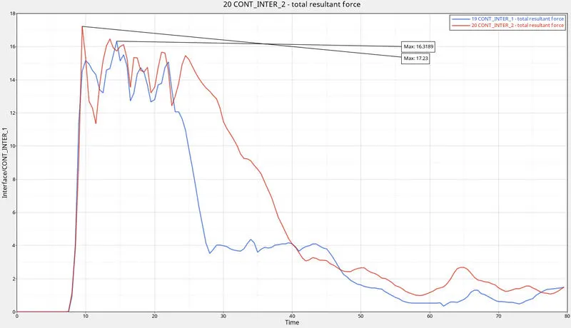
The Axial force will be zero till the vehicle touches the barrier due the gap in between. As soon as the bumper(which is the first part of the vehicle touching the Rwall)touches with the Rwall, there is a sudden rise in the force and reaching a maximum value of 17.23 KN for the left rail while the maximum value of the right rail has reached a value of 16.31 KN. Then it reduces with time as the contact of the elements within the rail get reduces and reaches a minimum value.
SECTIONAL FORCES:
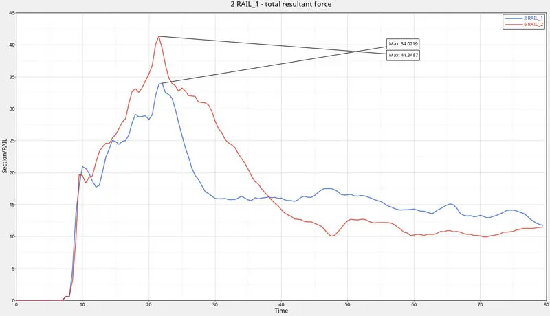
The plot indicates the forces or loads transmitted along both the rails of the vehicle.We can see that the left rail(blue)reaches a maximum value of 34.02 KN while the right rail(red) has a maximum value of 41.34 KN.This is because of the slight variation in the designs of the rail. The load transmitted along both the rails are very high at the initial stages of deformation and afterwhich it got reduced with slight reduction variation in each rail.
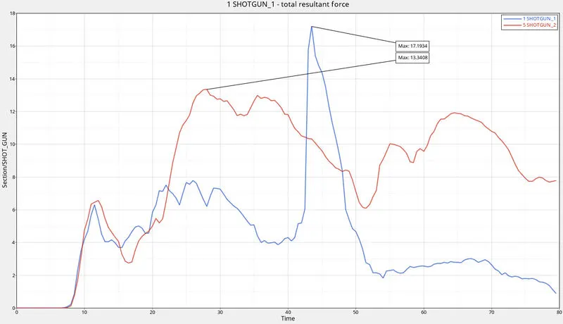
This plot indicated the load which has been transmitted through the shotguns of the vehicle. At the initial stage of deformation both the shotguns behave similarly. But at 20ms the right rail increases and reaches a maximum peak of 13.34 KN but the left rail does not have sudden peak till 40ms. After 40 ms the left shot-gun have a sudden peak and reaches a maximum of 17.193 and decreases suddently. The sudden peak is because the load transmitted or high force is transmitted at that time of deformation.
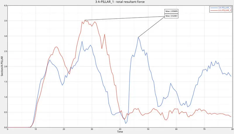
This plot indicated the load which has been transmitted through the a-PILLAR of the vehicle. The left A-pillar reaches a maximum peak value of 3.52 KN @ 46ms while the right rail reaches maximum peak value of 2.9 KN @ 27ms.This is because the load transmitted along both the A-pillars are slightly different. The left one varying load transmission but the right pillar decreases after its paek value.
ACCELEROMETERS:
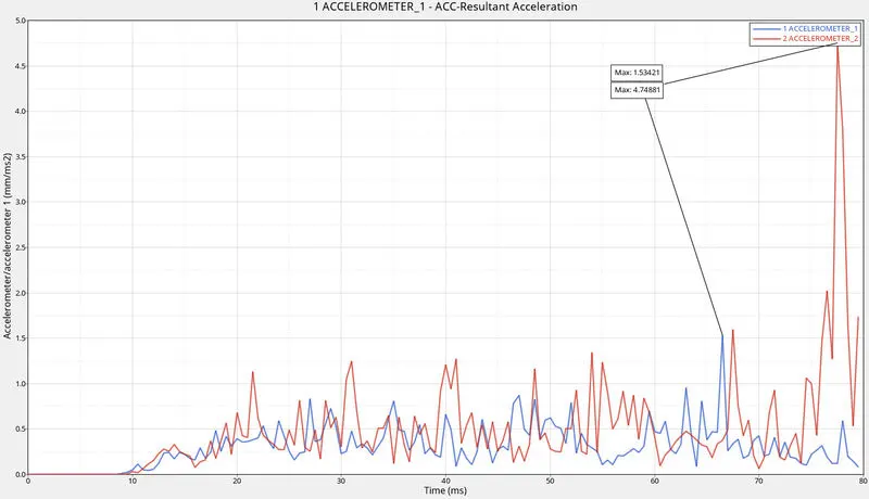
The graph shows the the acceleration happening on the simulation with respect to a node. Both the accelerometers have been transmitted same acceleration but at the end of the deformation the right rail have a sudden peak in its value to 4.74 mm/ms^2. This depends upon entire design structure on the right part of the vehicle. Whereas the left rail only reaches a peak value of 1.5 mm/ms^2. On the driver side more energy has been transmitted ie more vibration is transmited along it while on the passenger side more energy have been absorbed which means lesser vibrations along that portion.
INTRUSIONS ON DASH WALL:
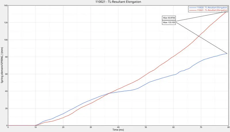
Intrutions are given inorder to understand the change in displacement happened b/w two nodes.This graph shows the intrusions happened in dash wall with the selected two nodes.
The spring elemets 110020 and 110021 corresponds to the node Id 66695 and 66244 respectivily.
The graphs shows that the first spring 66665 has intruded 83.97 mm into the passenger cabin, while the second spring 66244 has moved to value of 133.105 into the passenger cabin.
ENERGY ERROR AND MASS ERROR:
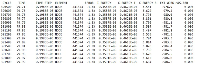
The energy error has reached to a value till -1.8% which is acceptable and the mass error does not have any change.
CONCLUSION:
The frontal crash has been inputted with the initial properties as given and the simulation is runned analused with the graphs plotted.
From the above results it can be concluded that the vibrations will happen higher in the right side of the vehicle than that of the left rail.
The forces transmitted along the rail and shotguns are much higher on the right side than that of the left side. But the force transmitted on the A-piller is higher on the left side.
At the initial stage when the bumper crashes and load transmitted to the rail is almost same on both ends and after which the load is distributed to different components.