FRONTAL CRASH OF NEON DODGE BIW USING RADIOSS

AIM:

To analyze, the frontal crash BIW of the car and observe the resultant output and energy plots from the simulation.

OBJECTIVE:

1. To check the unit system and either follow[Mg mm s] or [Kg mm ms].
2. To create an appropriate interface, friction 0.2 and recommended parameters.
3. Make sure of no penetrations and intersections.
4. To correct rigid bodies if any issues.
5. To create a rigid wall with friction 0.1.
6. To compare the model weight with the full-scale 300k nodes model and use added masses to reach target weight 700kg while getting CG about the required range.
7. To give an initial velocity of 35 mph.
8. Then use a model checker to ensure good quality.
9. Mention the time-step as 0.5 to 0.1 microseconds.
10. To run the simulation of frontal crash-BIW as 80 ms.

KEYWORDS: Rigid wall, Bumper, Accelerometer, Displacement, Rigid body, A-pillar, B-pillar, Cross-section.

SOFTWARE USED: Hypermesh and Hypercrash.

THEORY:

The objective of a crash test for Federal Motor Vehicle Safety Standard (FMVSS) No. 208 is to measure how well a passenger vehicle would protect its occupants in the event of a serious real-world frontal crash. This is sometimes referred to as the crashworthiness of a vehicle. This report reviews potential test procedures for evaluating frontal crashworthiness.

The ideal frontal crash test procedure will be able to evaluate occupant protection while ensuring that the vehicle will not jeopardize its crash “friendliness” with its collision partners. Finally, the test conditions (e.g., impact speed, impact angle, and test device) must be representative of the frontal crash environment to which passenger vehicles are exposed on the highway. The objective of a crash test for Federal Motor Vehicle Safety Standard (FMVSS) No. 208 is to measure the crashworthiness of a passenger vehicle. The standard specifies performance requirements for the protection of vehicle occupants in crashes. Historically, this has encouraged improvements to the vehicle structure and restraint systems to enhance occupant crash protection.

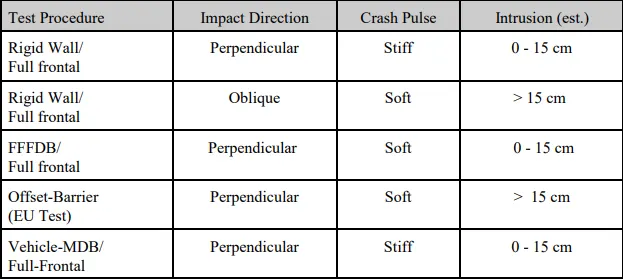
This report has addressed tests that assess the crashworthiness of a vehicle – the capability of a vehicle to protect its occupants in a collision. This is one aspect of crash compatibility. The other aspect of crash compatibility is aggressivity – the tendency of a vehicle to injure the occupants of the other vehicle in a vehicle-to-vehicle collision. This chapter examines the impact of each of the candidate test procedures on crash compatibility – particularly in frontal crashes. The specific objective is to determine whether the candidate test procedures would invariably result in a significant negative impact on safety that cannot be mitigated in a reasonable manner.
In general, the lack of crash compatibility arises from three factors:
• Mass Incompatibility
• Stiffness Incompatibility
• Geometric Incompatibility

Crash tests provide insight into the protection offered by the vehicle itself. As a secondary benefit, the published crash ratings encourage automakers to make ongoing improvements. But with two primary testing organizations (government and insurance industry), multiple tests conducted on each car, and competing manufacturer claims, it can be difficult to make sense of it all. This crash-test primer will enable you to understand the information that matters most.

Structural design and safety systems determine how well a vehicle protects its occupants. But it is only independent crash testing under controlled conditions that differentiates one car from another and tells us how well its key components work together. A crash test may reduce the vehicle to a shattered wreck, yet good structural design keeps passenger-space intrusion to a minimum. Important safety systems such as safety belts, air bags, and head restraints serve a vital role, by restraining, positioning, and cushioning occupants while a collision takes place.

The two independent crash-test information sources are the National Highway Traffic Safety Administration (NHTSA), a branch of the Department of Transportation, and the Insurance Institute for Highway Safety (IIHS), an independent safety-research group sponsored by auto insurers. Using different methodologies, both organizations conduct front and side-impact crash tests. In addition, NHTSA tests for rollover propensity and the IIHS evaluates rear-crash protection and roof strength.

Front crash

NHTSA's front-crash test accelerates a car straight into a rigid barrier at 35 mph, with the entire width of a vehicle's front end hitting the barrier. Instrument-bearing, seat-belted crash-test dummies in the two front seats record the level of crash forces on the head, neck, chest, and legs. Those measurements correlate with injury, but formerly only the head and chest results formed the basis of the star rating. Individual star ratings are assigned to the driver and the front passenger. Some automotive experts have criticized NHTSA's full-frontal, rigid-barrier test as unrealistic because such head-on crashes into a flat, solid wall are relatively rare. Others argue that real-world or not, flat-barrier testing is a good way to gauge the effectiveness of the restraint systems, primarily the safety belts and airbags.

PROCEDURE:
Set-up has to be followed,

• First, we want to import the neon_front file by using the import option and select the file that we want to import the data of file name as neon_front_0000.rad that is referred to as an input file of the simulation and click import. Now the file is imported and the import selection process and import file dialog box is shown below,

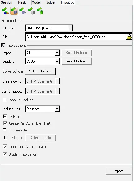
Fig: Import Dialog box

• After importing, the input file a model will open and that is shown below,

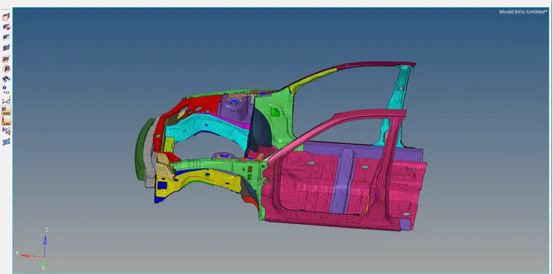
Fig: Open model

• Now check the unit system and verify that the same pattern of the unit system has followed in this simulation. It could be in either [Mg mm s] or [Kg mm ms] that are mentioned by the instructor.
• The unit system is required to obtain the resultant plots in that certain units. The unit system for this simulation is shown below,

Fig: Starter file

• After verifying the unit system to create an appropriate interface with the friction of 0.2 and using recommended parameters, Here there should be a default interface is present in the model that is shown below,

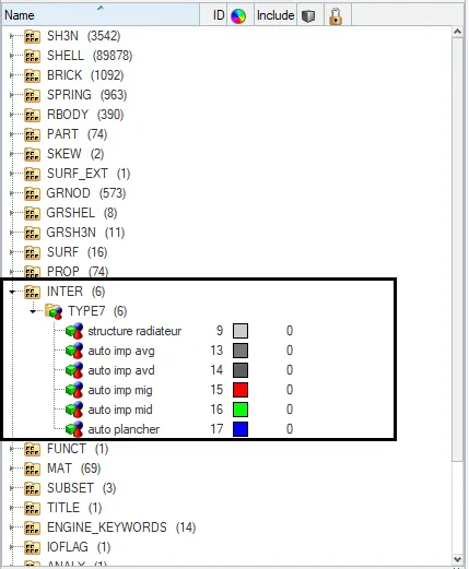
Fig: Solver table

• We are deleting the default interface(TYPE-7) that is present in this model because it indicates the group of different sectors of self contact in the vehicle. we want to create the total self contact of the BIW body of the vehicle.
• Therefore create the interface of Type-7 by selecting the solver>inter>right click inter>select create and enter the recommended parameters in that properties card. Type-7 interface is using because it is nodes to surface contact.

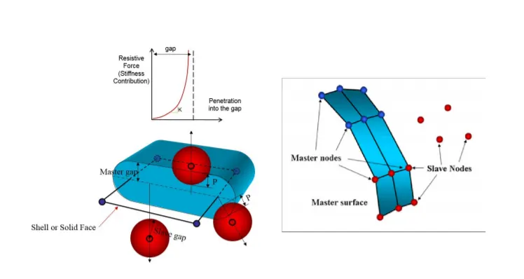
Interface Type 7: Nodes to Surface Contact

1. Automatic node to surface contact interface using the penalty method with variable stiffness
2. A gap is defined around the master segment and the slave nodes
3. The contact gap can be constant or variable
4. Resistive forces are applied to keep slave nodes out of the contact gap
5. The interface time step is computed to insure stability
6. Interface type 7 is a general-purpose interface and can simulate all types of impact between a set of nodes and a master surface. Contrary to interface types 3 and 5, interface type 7 is non-oriented and slave nodes can belong to the master surface. Therefore, this interface can simulate auto-impact, especially buckling during a highspeed crash. Interface type 7 solves all problems and limitations encountered with interface types 3 and 5. The search for the closest segment is done via a direct search algorithm; therefore, there are no search limitations and all possible contacts are found. The energy jumps induced by a node impacting from the shell edges are removed by the use of a cylindrical gap around the edges.

IMPORTANT INTERFACE PARAMETERS:

Igap - Determines how the size of the gap is calculated.

Gap_min - Minimum gap for activation of the interface.

Inactiv - Action to take if initial penetration exists.

Istf - Affects how the stiffness of the interface is calculated.

Iform - Friction formulation

St_min - Minimum stiffness to use in the interface.

Idel - What do with slave nodes and master segments if an element fails(deleted) that they are attached to.

• Here the recommended parameters for the type-7 interface and the friction of 0.2 that we entered are shown below,

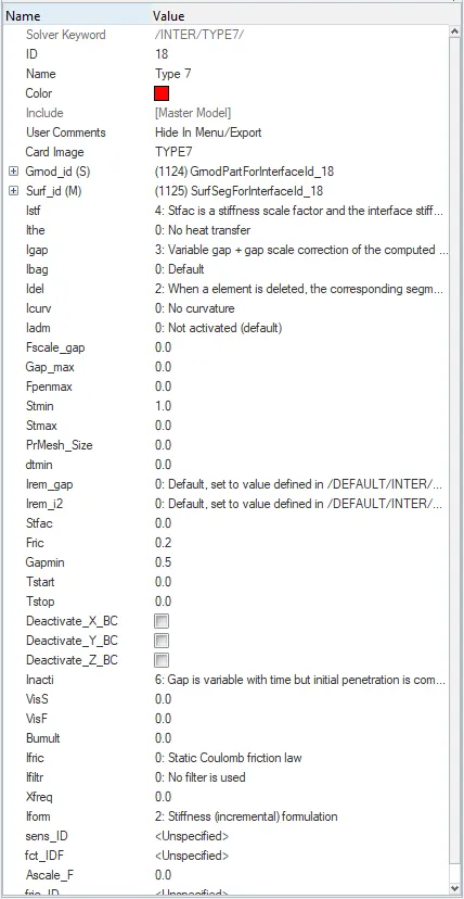
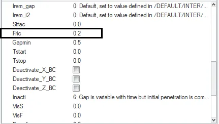
Fig: Selfcontact interface recommended properties

• Now check the penetration and intersection for the whole body of the vehicle by selecting tools>penetration check>select the group in the selection and click check to verify the group whether the penetration occurred or not.
• After checked the penetration it resultant that any occurred or not, hence this group is cleared from the penetration and intersection that is shown below,

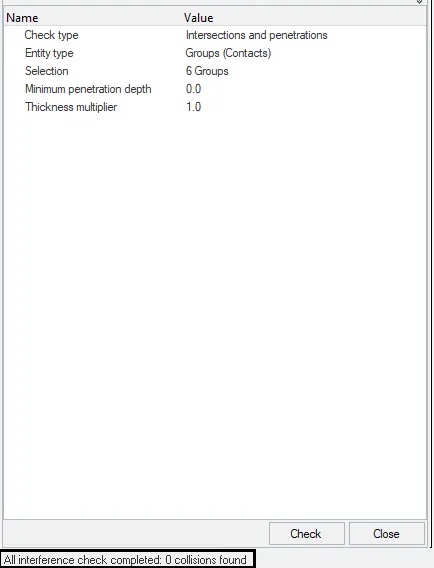
Fig: Penetration Check

• After verifying the penetration and intersection we want to check the rigid bodies by using the model checker option and if any issues may appear then clear that errors. In this model, there are no issues occur.

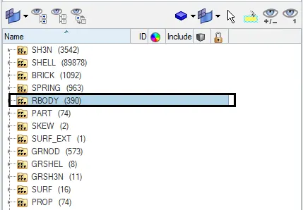
Fig: Rigid body

• Then create a rigid wall to crash the vehicle in a rigid plane(Crash Simulation) and observe the simulation and energy between the wall and vehicle. Right-click the solver>create>RWALL>select plane>enter the properties of a rigid wall of friction as 0.1 and the Dsearch as 2000. Select the engineering data and ensure the axis of XM, YM, ZM which denotes the vehicle movement from normal to a rigid wall. In XM axis we are selecting the vehicle bumper portion
• And in normal N we initiate the distance between the rigid wall and the vehicle bumper.
• Therefore the RWALL properties and the data's given in this simulation are shown below,

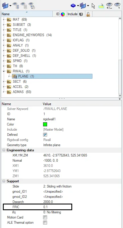
Fig: Rigid wall properties

• A created rigid wall of friction as 0.1 and the frontal area is shown as below,

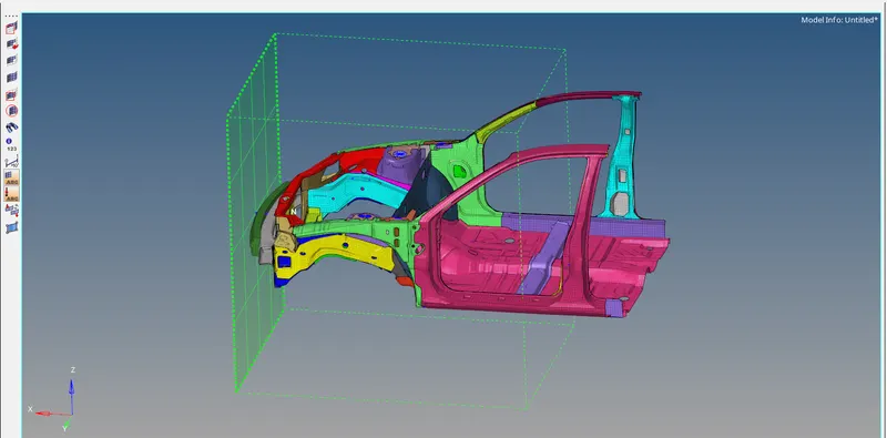
Fig: Frontal car with rigid wall

• Now we want to move the CG in the required range by adding the mass for each node and to create the excess mass for certain selected nodes that is depends upon the movement of CG.
• Ensure that CG should present between the center of the driver seat. First, we verify that the actual total mass present in nodes by selecting the mass>balancing option in hyper crash. Before that, import the edited file which is worked on hypermesh into the hypercrash.
• Here the actual total mass value shows as 188kg for 300k nodes. To view, the CG click the overview option and view the model it will show the CG as a dot point. That value is shown as below,

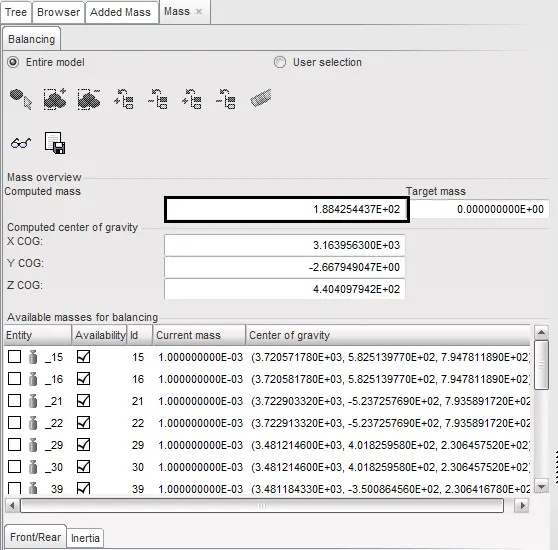
Fig: Default Mass

• To move the CG increase the mass value from 188kg to 700kg that value is mentioned by the instructor. By selecting loadcase>added mass> it shows the total nodes and the mass value for those nodes. Those values and separation of nodes are set as default. The selection of added mass is shown below,

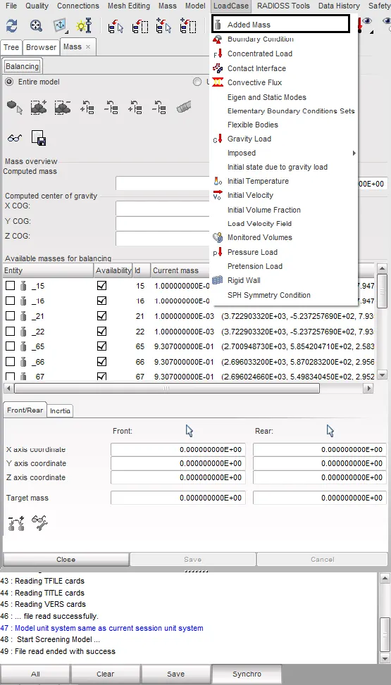
Fig: Added Mass

• In the added mass, click box icon it shows 8 different types that depend upon the distribution of mass with group or node. Here select Type=1(mass is distributed to each node of a node group) it will create a section, in that section enter the mass value to add total mass value in the frontal area of a vehicle.
• By balancing the mass value and creation of mass section will move the CG at the required point. The type selection of added mass is shown below,

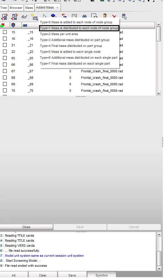
Fig: Mass type

• Therefore the mass is added through the mass type and 8 sections are created each section contain some amount of additional mass added in particulars node that is selected by the user. Now added mass section and the selected nodes are shown as below,

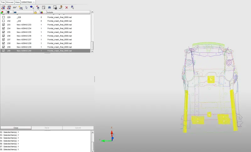
Fig: Section added mass

• Now the total mass is reached as 700kg by adding the new mass value for some specified nodes and that value is initiate below,

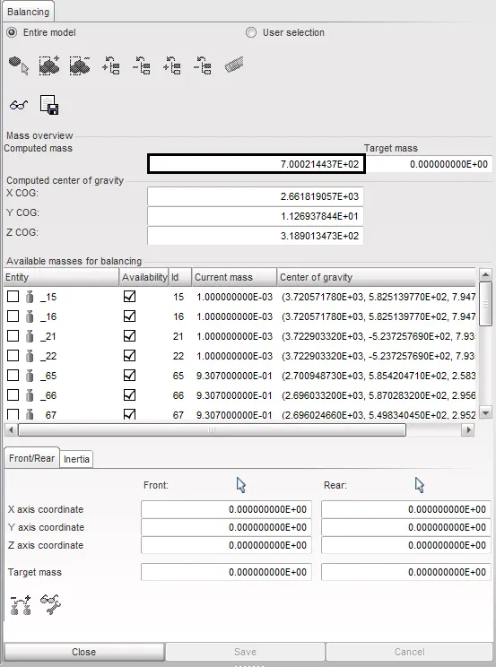
Fig: Value-added mass

• By changing the mass of 700kg the CG has reached a required range that is in between the driver seat and B pillar. Mass balancing is used to change the mass value and to move the CG by adding the mass in different valid nodes. Hence CG is moved and that is shown as below,

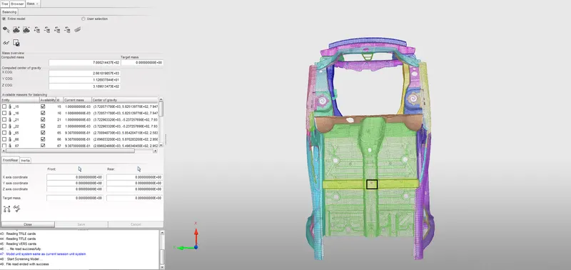
Fig: Centre gravity point

• Now we want to give the initial velocity of a vehicle as 35mph that is given by the instructor. By right-click the solver>create>INIVEL> setup the properties by giving the value of velocity as 15.65mm/ms it is obtained by converting the unit of 35mph. Then click the gmd_ID and select the groups and confirm it.
• Therefore the initial velocity is created and that is shown as below,

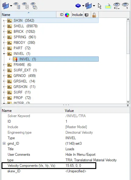
Fig: Initial velocity

• After creating an initial velocity check whether the model is in good condition or not by using the model checker option. Select Tools>model checker>click run icon it will checks the total model and show the results. If any errors will appear after the completion of model checker clear the errors to run the simulation. Here the model checker is run completely and that is shown below,

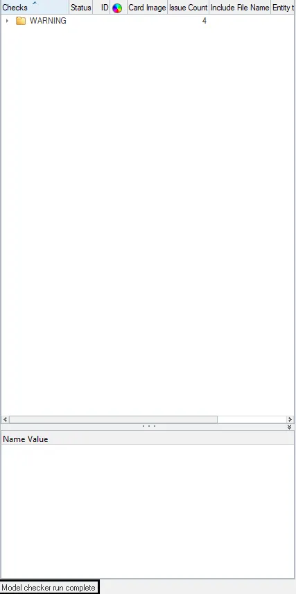
Fig: Model checker

• To mention the time step as 0.5 to 0.1 microseconds by selecting the solver>engine keywords>dt/noda and enter the value of Tmin in that setup table as 0.0001. And to set the run time of simulation as 80ms by selecting solver>engine keywords>run>Tstop and enter the simulation run time. The time step and run time setup data are shown below,

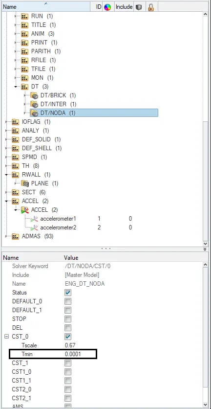
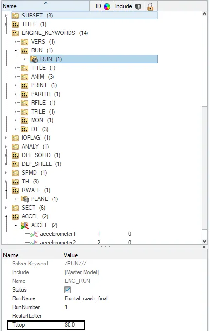
Fig: Timestep and Run time properties

OUTPUT REQUEST:

SECTIONAL FORCE:

• After edited all the setup for simulation then we have to set the output request that depends upon what the output we want in that simulation. Here we want to obtain the Sectional force in the rails at the location of indicated node 174247 and parallel opposite side node.
• To create the cross-section by selecting the solver>create>SECT> then we want to create a movable frame in that cross-section and select nodes of origin, X-axis, and XY axis to obtain the normal N direction opposite from the crash direction X. This frame is created to the analysis of F3 force that is normal Z here they are considered as a sectional force while on the crash simulation.
• The below image shows the recommended nodes for sectional force and the created two frames

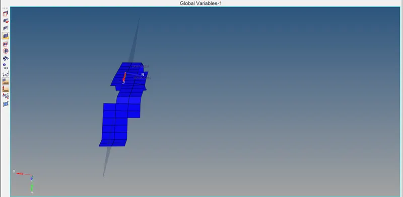
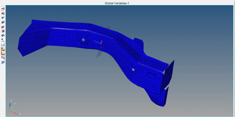
Fig: Cross-section

• We want to initiate the system in section property and to mention the system number in Frame_ID of each recommended section. The cross-section for sectional force in the particular node and the frame id is shown as below,

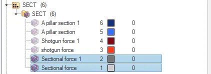
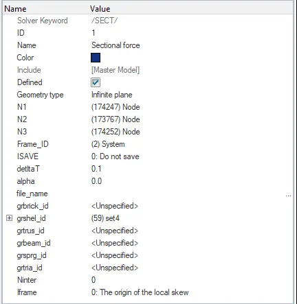
Fig: Cross-section properties

• In a movable frame, we want to select the origin node(N1), axis node(N2), and plane node(N3). The same node intimate in the system is required in the section node ID.
• A node selection and the axis point for the sectional force is shown below,

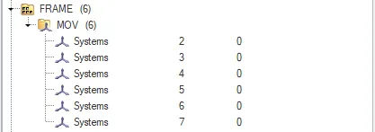
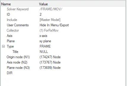
Fig: Frame Properties

AXIAL FORCE:

• Here we want to obtain the output request for axial force received on the rails from the bumper so create the interface group(type-7) for rail and bumper with recommended properties. By selecting the Model>right click and select the create >contact it creates a group and edit the group with the recommended parameters.

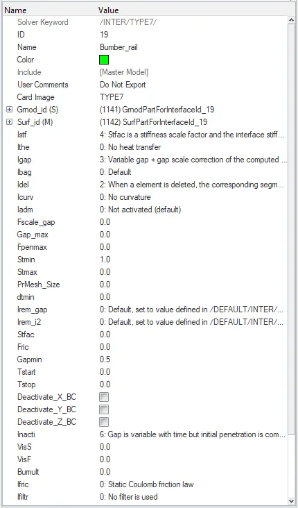
Fig: Interface recommended properties

• Select the master nodes as bumper and the slave nodes as rail and other parameters are mentioned as recommended type-7 parameters. Denote the output block for Bumper rail group to obtain the axial force received on the rails from the bumper. The master and slave node for this group is shown below,

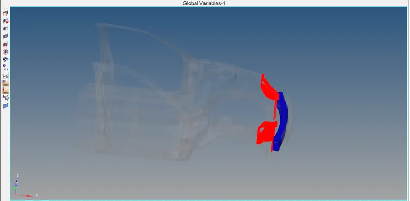
Fig: Master and Slave nodes

SHOTGUN CROSS-SECTIONAL FORCE:

• To create the cross-section by selecting the solver>create>SECT> then we want to create a movable frame in that cross-section and select nodes of origin, X-axis, and XY axis to obtain the normal N direction opposite from the crash direction X. This frame is created to the analysis of F3 force that is normal Z here they are considered as a sectional force while on the crash simulation.
• We want to initiate the system in section property and to mention the system number in Frame_ID of each recommended section.
• In a movable frame, we want to select the origin node(N1), axis node(N2), and plane node(N3). The same node intimate in the system is required in the section node ID.
• The below image shows created shotgun force and frames

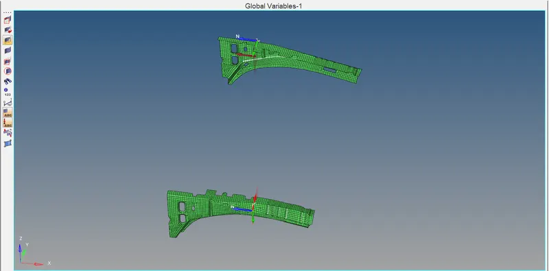
Fig: Shotgun cross-sectional force

A-PILLAR CROSS-SECTIONAL FORCE:

• To create the cross-section by selecting the solver>create>SECT> then we want to create a movable frame in that cross-section and select nodes of origin, X-axis, and XY axis to obtain the normal N direction opposite from the crash direction X. This frame is created to the analysis of F3 force that is normal Z here they are considered as a sectional force while on the crash simulation.
• We want to initiate the system in section property and to mention the system number in Frame_ID of each recommended section.
• In a movable frame, we want to select the origin node(N1), axis node(N2), and plane node(N3). The same node intimate in the system is required in the section node ID.
• The below image shows the created A-pillar cross-sectional force and frames,

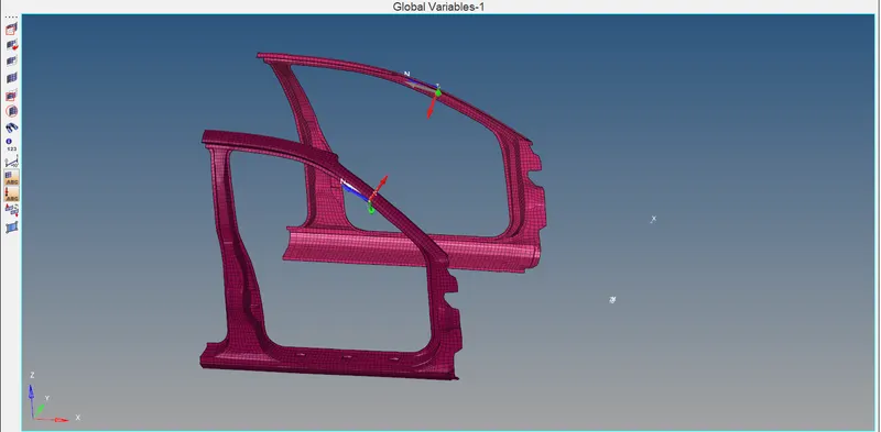
Fig: A-pillar cross-sectional force

• Here all the cross-sections and the frames are shown below,

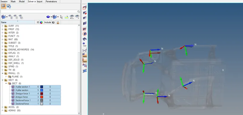
Fig: Cross sections and frames

ACCELEROMETER:

• Here we want to observe the output of the acceleration curve received on the accelerometer at base of B pillar. By selecting the solver>right click and select create>ACCEL it will create acceleration now select Entity IDs and pick one node in the base of the B-pillar.
• It creates an accelerometer for that node in B-pillar to analyze the acceleration curve for that node. The same procedure is followed for the opposite node of B-pillar hence it created and that are shown below,

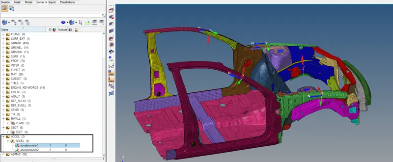
Fig: Accelerometer points

INTRUSIONS:

• To create the Intrusions on the dash wall at nodes of 66695 and 66244. By selecting the solver>TH>node> and click the select Entity IDs and right-click on the node selection tab and enter the node number it will consider that node for output observation.
• The same procedure is followed for the 66244 node hence it is created and that is shown below,

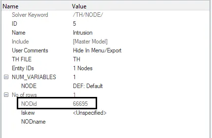
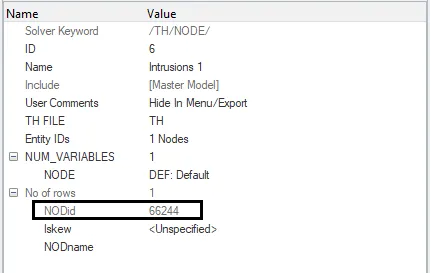
Fig: Intrusion properties

• Intrusions on the dash wall nodes 66695 and 66244 are intimated below,

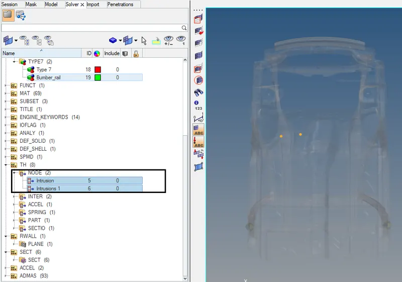
Fig: Intrusion nodes

• Before running the simulation check whether the model is in good condition or not by using the model checker option. Now import the model into hypercrash and select quality>model checker>click run icon it will checks the total model and show the results. If any errors will appear after completion of model checker, clear the errors to run the simulation. Here the model checker is run completely and that is shown below,

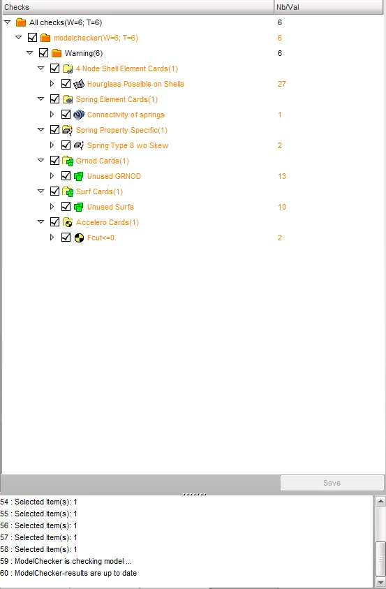
Fig: Model checker

OUTPUT PLOTS:

• Now the result is obtained in the respective given folder, open the folder, and analysis the errors like energy error and mass error. These errors are shown in the Engine Out file that is shown below,

Fig: Energy error and Mass error

• Here the result shows the two errors, energy error as -2.5 % and mass error as 0.000 %. An energy error should be in -5% is considered as better for simulation.
• The total number of cycles and the simulation time also noticed in that output and the values are shown below,

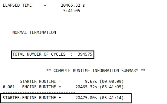
Fig: CycleTime

• Now open the hyper view and load Frontal_crash_final.h3d model file and select the apply option to open that model in hyper view. Therefore the model is opened and now to change the result type as Von Mises(s) to get the Von Mises Stress Contour Plot select the components and edit the averaging method as simple and click apply to get the animation of the vehicle crash on a rigid wall.

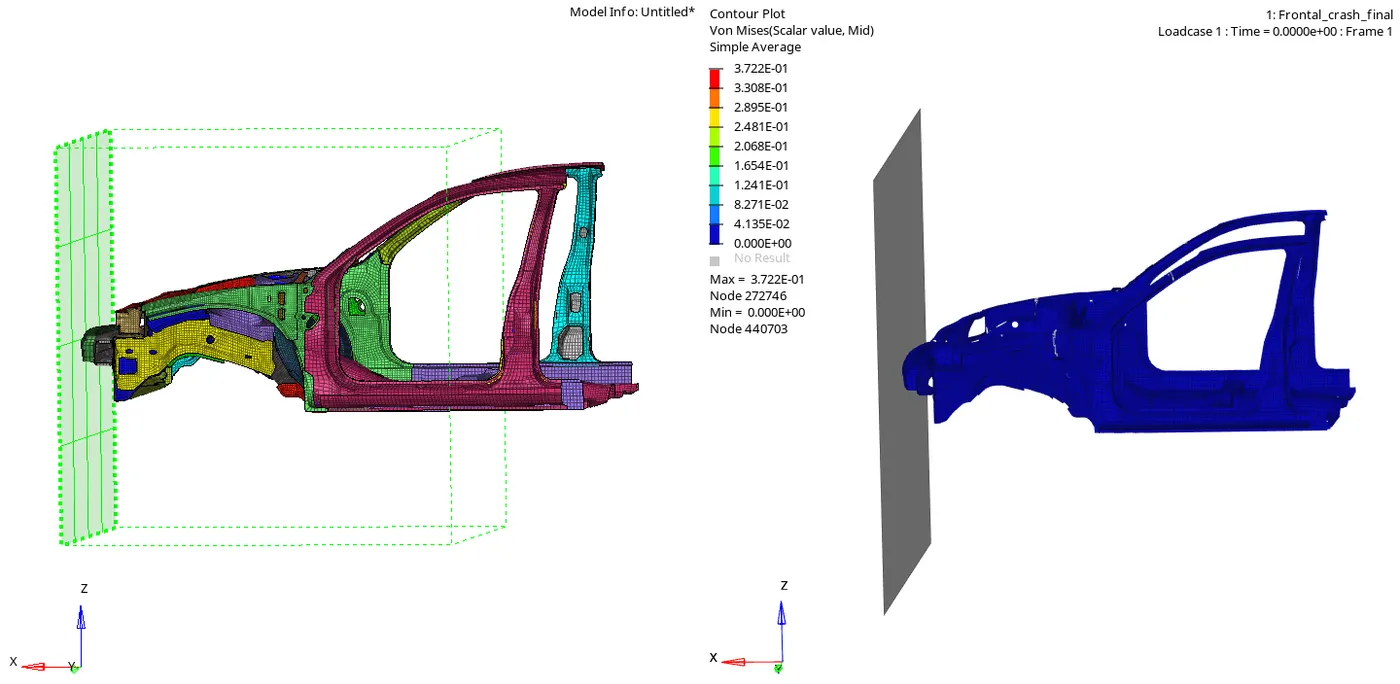
Fig: Open model Vonmises stress Contour Plot

• Now the contour plot is generated click the mesh icon to visualize the deformation of elements in each node. Here if you see in the plot contour above is Von Mises stress, here the component going to crash with time as we run our simulation. It shows a different range of colors as stress increases on the component. Von Mises stress is a value used to determine if a given material will yield or fracture. It is mostly used for ductile materials, such as metals. Von Mises stress is computed and compared to the yield stress material. If the von mises is smaller than the yield stress the computed stress is the one used in order to compute the internal force of the element. The minimum and the maximum value of stress is shown as below,

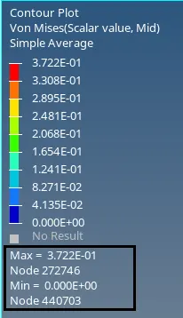
Fig: Stress value

ENERGY PLOTS:

• To create the plot for each energy and absorbs that what was happening during the crash and how could the element gets deforming while applying some force. Now select hyperchart option that will give the empty graph as a display. Import the file Frontal_crashT01 and click the apply option.

SECTIONAL FORCE:

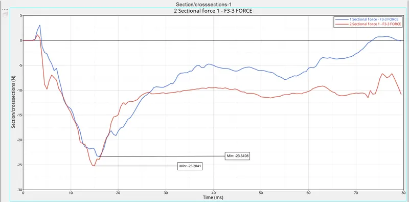
Fig: Sectional force plot

From the above graph, we are observing the sectional force that is created in the rail of the required node of 174247 and the parallel side node. A cross-section is created to observe the force during the crash of a vehicle the direction is defined by the moving frame through normal Z direction.

Each cross-section represents each skew system that should be indicated in that cross-section properties.

The graph shows that the maximum sectional force obtained in node 174247 is 23.3408Kn at the time of 17ms. In this result, the force we obtained is irrespective of the direction. Thus force acted on the rail of node 174247 is acted negative that should depend upon the moving frame of the cross-section.

The sectional force 1 results show the other side node of the rail as opposed to the 174247 node. The maximum sectional force obtained in this node is 25.2041Kn at the time of 15ms. In this result, the force we obtained is irrespective of the direction. Thus force acted on the rail of this node is acted negative that should depend upon the moving frame of the cross-section.

By comparing with these two sectional forces a sectional force1 gets the maximum force obtained on rails during the crash of vehicle is 25.2041Kn at the time of 15ms this may depend upon the value-added mass in the vehicle.

AXIAL FORCE:

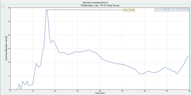
Fig: Axial force plot

The above graph shows the axial force received on the rails from the bumper during the crash simulation. It is obtained by creating the interface between the rails and bumper in that interface we are giving the master as bumper and slave as rails.

The axial force is observed when the frontal area is crashed on as rigid wall the slave is impacting with the master node and that force is obtained here. The maximum axial force is observed in this simulation is 29.2268Kn at the time of 17ms. The recommended parameters of the type-7 interface are executed for this simulation.

Due to the contact interface between the master and slave nodes the axial force is observed from the rail in this plot.

SHOTGUN CROSS-SECTIONAL FORCE:

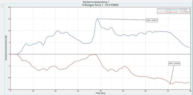
Fig: Shotgun cross-sectional force plot

From the above graph, we are observing the Shotgun cross-sectional force that is created on the parallel side of the shotgun part in the vehicle. A shotgun cross-sectional force is created to observe the force during the crash of a vehicle, the direction is defined by the moving frame through normal Z direction.

Each cross-section represents each skew system that should be indicated in that cross-section properties.

The graph shows the maximum value for one side of the shotgun force is 15.0417Kn at the time of 38ms and the other side is 12.6218Kn at the time of 72ms this difference may appear due to the node differences and the frame direction acted on the force. In this result, the force we obtained is irrespective of the direction so positive and negative value is not considered it will change through the movement of the frame during crashing.

By comparing with these two shotgun sectional forces left side shotgun obtained more force of 15.0417Kn compared with the right side shotgun force 12.6218Kn this may depend upon the value-added mass in the vehicle.

A-PILLAR CROSS SECTION:

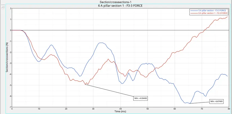
Fig: A-pillar cross-sectional force plot

From the above graph, we are observing the A-pillar cross-sectional force that is created on the parallel side of the A-pillar in the vehicle. A shotgun cross-sectional force is created to observe the force during the crash of a vehicle, the direction is defined by the moving frame through normal Z direction.

Each cross-section represents each skew system that should be indicated in that cross-section properties.

The graph shows the maximum value for one side of the A-pillar force is 4.93482Kn at the time of 28ms and the other side is 6.67481Kn at the time of 65ms this difference may appear due to the node differences and the frame direction acted on the force. In this result, the force we obtained is irrespective of the direction so positive and negative value is not considered it will change through the movement of the frame during crashing.

By comparing with these two A-pillar sectional forces left side of A-pillar obtained more force of 6.67481Kn compared with the right side of the A-pillar force 4.93482Kn this may depend upon the value-added mass in the vehicle.

ACCELEROMETER:

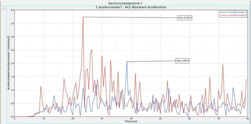
Fig: Accelerometer plot

The accelerometer is observed in each B-pillar of the vehicle by selecting the base node of two pillars and include the node for output blocks to find the accelerometer in each pillar. The above graph shows that accelerometer 1 and accelerometer 2 are stable up to 7ms and it gets raising after 10ms. The minimum point of accelerometer1 is 2.0613mm/ms^2 at the time of 38ms and the maximum point of accelerometer2 is 3.73613mm/ms^2 at the time of 23ms.

These differences between the accelerometer1 and accelerometer2 have appeared due to the deformation of elements and the added mass during CG.

By comparing with the accelerometer1 and accelerometer2 the maximum peak is observed in the accelerometer2 as the value of 3.73613mm/ms^2.

INTRUSIONS:

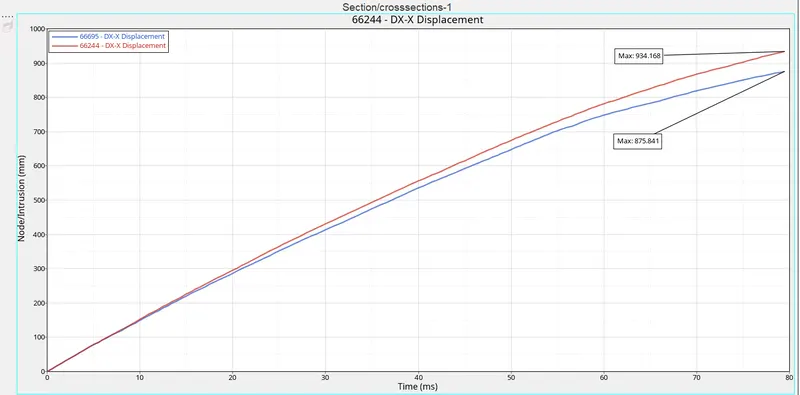
Fig: Intrusions plot

• The intrusion is the process of identifying the displacement of some reference point or line or node. Here we are calculating the displacement of two nodes in dash wall such as 66695 and 66244 are there node ID. The nodes are selected and the above graph shows the two displacement points of those nodes.
• The maximum displacement point in node 66695 is 934.168mm at the time of 78ms and the maximum displacement point in node 66244 is 875.841mm at the time of 78ms.
• Observation of the graph shows that the displacement acting on 66695 node is less when comparing with 66244 node.
• By comparing with two nodes the node 66244 takes more displacement during the crash simulation.

ENERGY PLOTS:

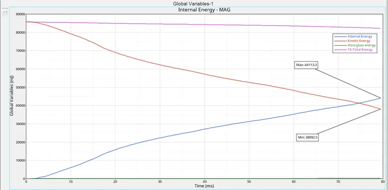
Fig: Energy plot

• The above energy plot shows that increase in internal energy while the frontal area of the car is crashed on the rigid wall because of the contacts in the element it's getting raised, up to the simulation runtime when it completes the internal energy rises also getting stopped that will depend upon the deformation of the elements during a crash simulation. When the internal energy is observed due to contact of the car and a rigid wall. During the crash, there is a velocity is acted along with the car and it creates some energy that is observed as internal energy.
• During the crash simulation, the internal energy is getting raised up to 44113.3mJ at the time of 78ms and at that stage kinetic energy also occurring between the car and the rigid wall. There is a decrease in kinetic energy flow of 38092.5mJ at the time of 78ms because the velocity of the car is acted in a rigid wall that increases the internal energy so kinetic energy is decreased at the same level.
• The total absorption of energy is obtained when the car is crashed on the rigid wall and that energy is represented as total energy = sum of internal energy and kinetic energy. By equating the internal energy and the kinetic energy the total energy will remains in constant flow but here there should be a slight variation is shown in total energy because of the hourglass energy present during the crash simulation.
• Hourglass energy is observed in this graph that changes the total energy flow but here hourglass energy is observed as a very minimum value therefore it is negligible and it won't affect the total energy as more.

CONTACT ENERGY:

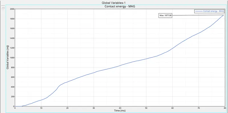
Fig: Contact energy plot

• A Penetration by the contact force is defined as contact energy here the contact energy is absorbed during the vehicle crashing on the rigid wall it will get deformation of elements and the penetration is also appear in the crash simulation.
• The force is created between the master and the slave node during the penetration that force and penetration are calculated as contact energy.
• Here the contact energy reaches the maximum point of 1877.08mJ when the time of 78ms.

TOTAL OUTPUT PLOTS:

• Therefore the total output plots are plotted and they are shown as below,

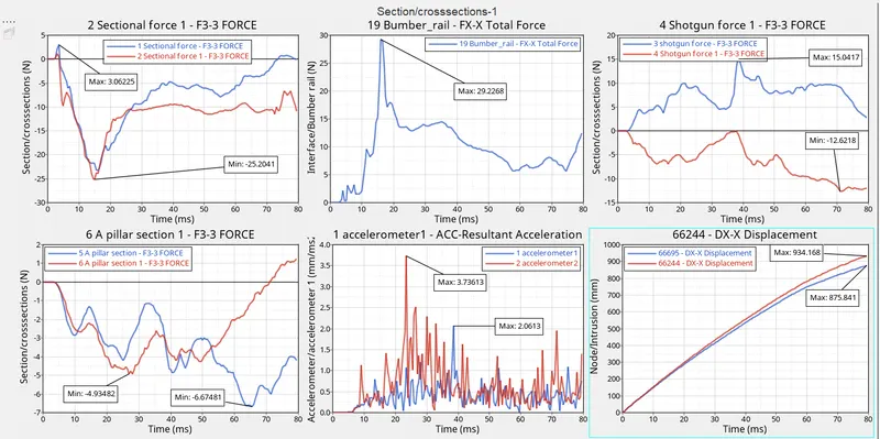
Fig: Total energy plots

LEARNING OUTCOME:

• Setup the model and create the card and their properties for frontal crash analysis using Hypermesh, Radioss, and Hypercrash.
• To know the types of force needed to calculate during the analysis.
• Analysis of energy plot after a frontal crash simulation is done.

CONCLUSION:

Hence the frontal crash simulation is done and has obtained the output plots for sectional force in the rails, axial force received on the rails from bumper, shotgun cross sectional forces, A pillar cross section, acceleration curve, and the intrusions on the dash wall. Therefore the frontal area of the vehicle is crashed on a rigid wall hence energy error observed in this simulation is -2.5 % and mass error as 0.000 %.

Energy plots show the variable energy observed during the crash simulation and they are analyzed.

A crash of frontal car with a rigid wall and their impacts, forces, and intrusion values are obtained from simulation resultant plots so the study is finally done.