Assignment 5-RADIOSS Interfaces & Study of Effect of Notches Challenge

Questions:

• Create the mesh for bumper assembly, mesh size should be 6mm. 

1. Run the crash tube model as it is.
2. Change the Inacti=6 and run.
3. Create the type 11 contact and run.
4. Remove both notches and remove the boundary condition on the rigid body node then run.
5. Create a new notch in the middle, select the whole section, and run.
6. Create a new notch with nodes only from opposing 2 faces and run.

Model 1 :- Meshing of bumper assembly

 

1. Import given model into hypermesh

• To Open the .hm file, Go to the File menu in the Standard menu bar >> Click Open >> Click Model >> Select the model to open >> click
• The model is displayed in the Graphics Area.
• 2. Assign quality parameters :-
  • To give the Criteria, Click on the Preferences in the Standard Menu bar >> Click Criteria Menu Settings >> Give Target Element Length as 6mm >> Click Ok.
  • The Criteria are given.
  3. Meshing:-
  • To perform a mesh, Select the Auto Mesh option from the 2D panel >> Click the Surface to mesh >> Give the Element size as 6 >> Click Mesh.

• The Mesh is completed and the model is made sure that there are no tria elements in the model.

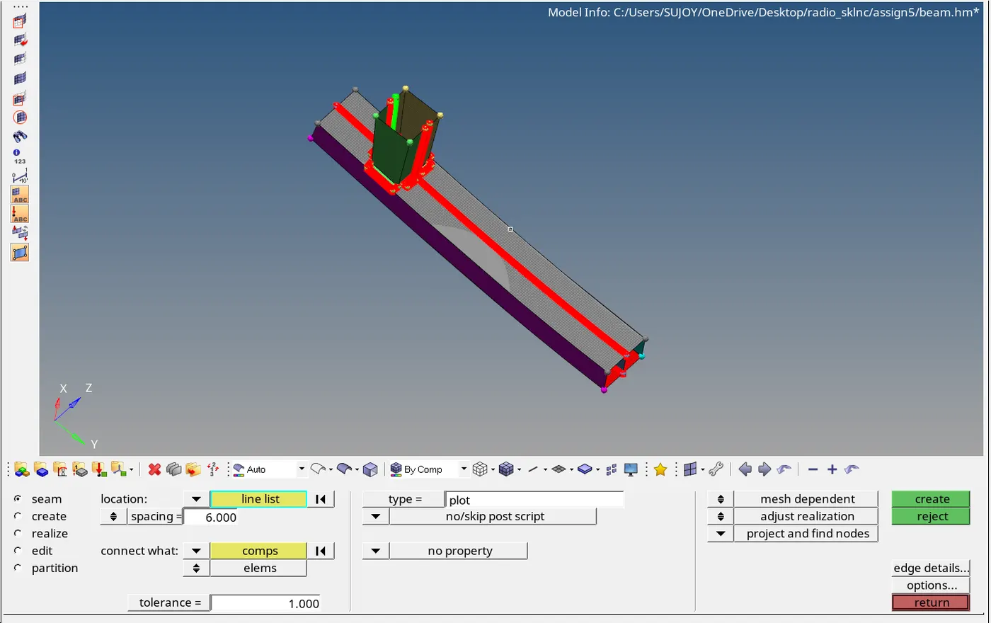
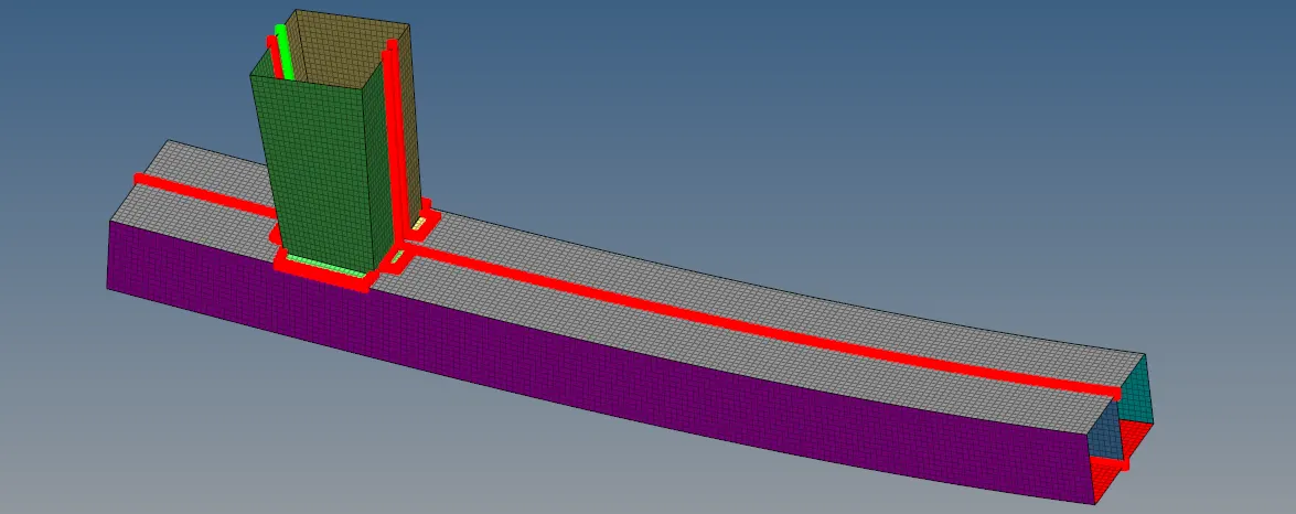
b. We have to connect the crash box and rear bumper, so as to give accurate result when we perform the analysis. There are different types of connections are available, apart from this we have chosen seam weld which is used to connect the two different materials. The below diagram shows the seam connection between the crash box and rear bumper.

Model 2 :- Solving different cases on crash tube

Case 1. Run the crash tube model as it is.

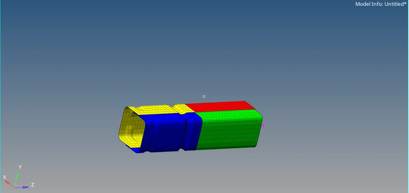
• After the Model is imported, The Simulation needs to be performed without changes in model in this case.

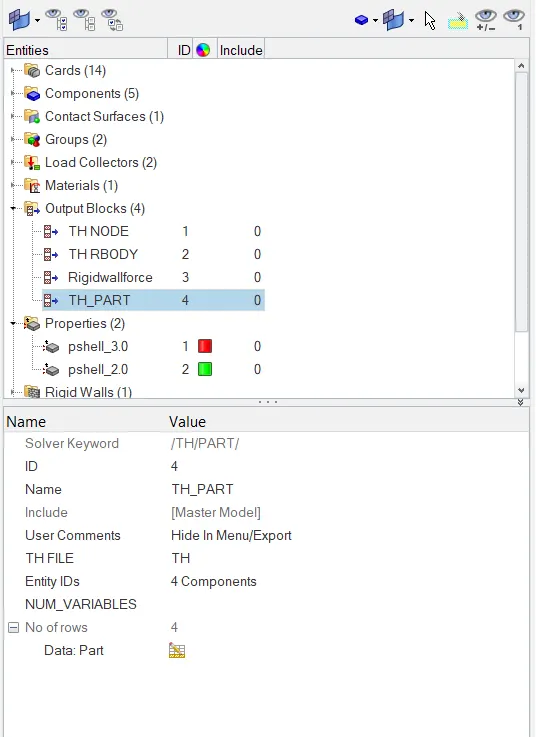
• In order to create the THPART we have to click on the output Blocks and create the TH PART , in entity id instead of nodes keep components and select all four components and click on ok. Then the TH part is created.

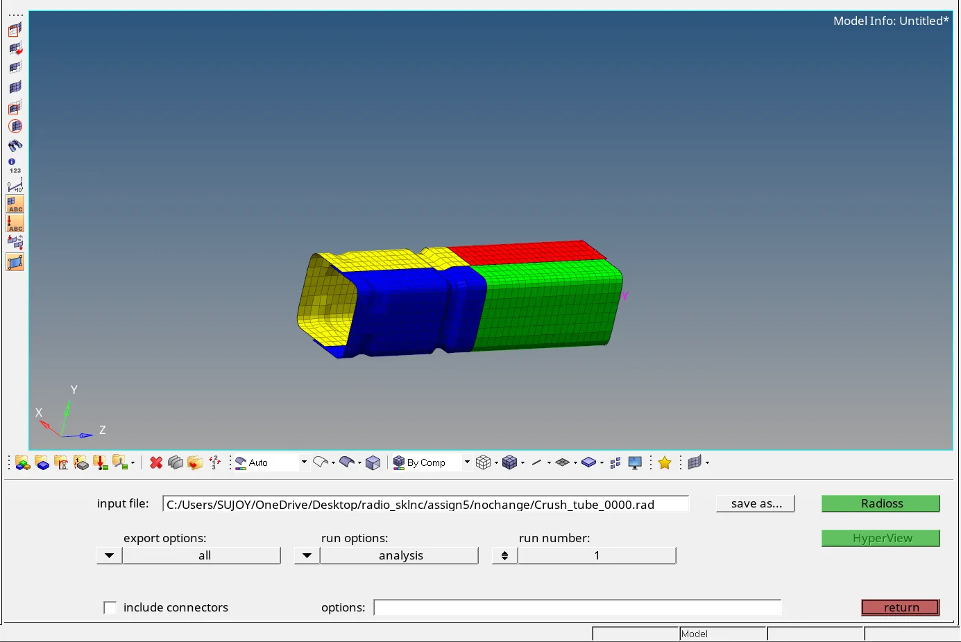
• To simulate the model, Go to the Analysis tab, Select the Radioss option > Select the location to save the file > Check include collectors box > In the options tab, type “-nt 4” > Click Radioss.

Open hyperview to view animation and contour plots from H3d file. 

• Click on view Results, which will open Hyperview window.

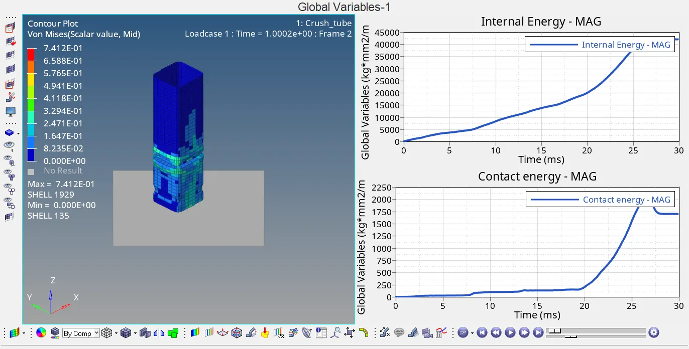
• In this simulation we can see that the tube starts to bend at the upper notch where the initial plastic strain occurs, and eventually the tube starts to bend at the lower notch. We can also observe that the tube fail between the notch region and then the region above the notch is crushed.
• The maximum Von misses stress and the maximum Plastic strain is formed at the corner section of the tube. 
• Open Hypergraph 2D and load T01 file.
• Go to GLOBAL VARIABLES > INTERNAL ENEGRY, KINETIC ENERGY and TOTAL ENERGY > MAG > APPLY. This will plot the energy graph.
• The Kinetic energy having higher value at the start of the simulation eventually starts to reduce with time as it gets converted into Internal energy, because the can is being crushed. Thus, the total energy remains constant with respect to time, but we can see a slight drop in energy at time equals to 25ms. This is because the tube is totally crushed and the energy is lost to the friction between the elements.
• Go to GLOBAL VARIABLES > CONTACT ENERGY> MAG > APPLY. This will plot the energy graph.
• The Kinetic energy having higher value at the start of the simulation eventually starts to reduce with time as it gets converted into Internal energy, because the can is being crushed. Thus, the total energy remains constant with respect to time, but we can see a slight drop in energy at time equals to 25ms. This is because the tube is totally crushed and the energy is lost to the friction between the elements.
• Go to GLOBAL VARIABLES > CONTACT ENERGY> MAG > APPLY. This will plot the energy graph.
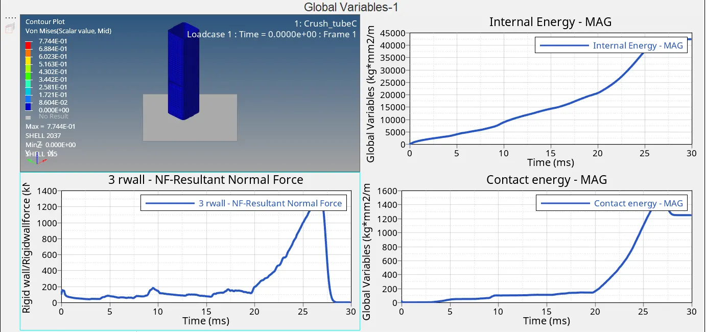
• The contact energy increases initilly at a slow pace and rapidly between 20 to 26 ms, because after 20 ms the tube deformation is completed and the force is crushing the surface of the tube in the formation of the folded layers. Here, the corner surfaces come in close contact of each other, resulting in the spring formation to repell the surfaces from intersecting each other. 
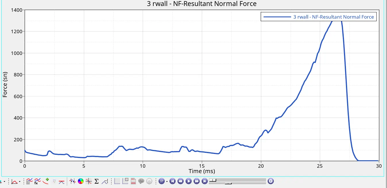
• Go to GLOBAL VARIABLES > RWALL > NORMAL RESULTANT, TANGENT AND TOTAL FORCES > APPLY. This will plot the rigid wall forces.
• A pattern is observed in the Resultant normal force, where a small amount of force increases at a regular interval of time. This increase in the force is when the corner edges fold the tube and the slave nodes try to penetrate into the master surface, the spring stiffness increase the force to oppose the slave node. After 20 ms we see a greater rise in the force value as the tube is crushed and more no of nodes come closer. Then the force is reduced and reaches to zero value.

• In Hyperview go to CONTOUR > RESULT TYPE > VON MISES > AVERAGING METHOD > SIMPLE > APPLY.

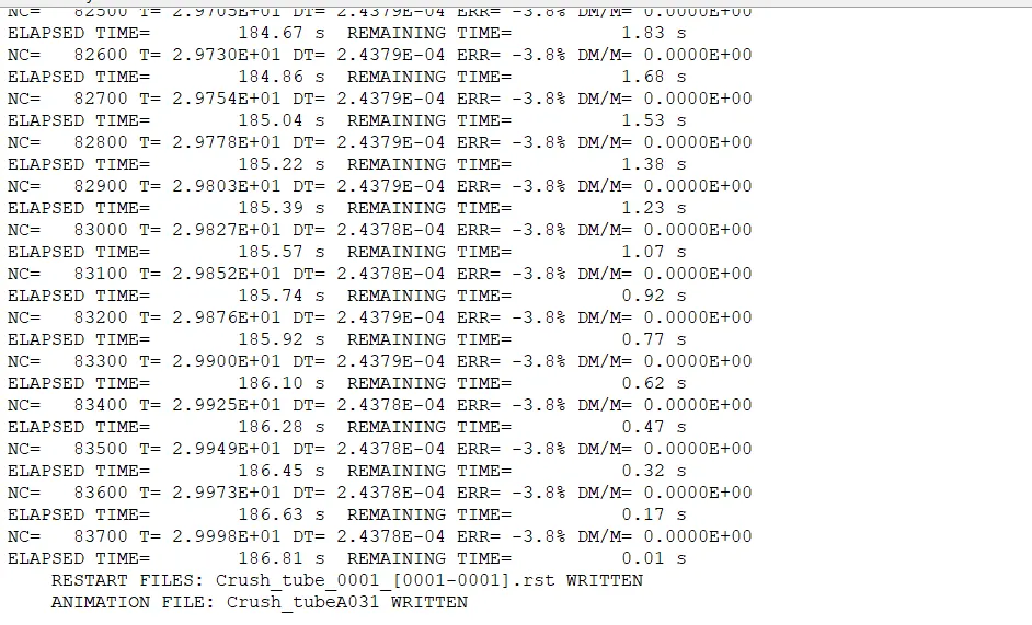
• From output file energy error is -3.8%% and mass error is 0% which is less than -15% to 2% and 1% respectively, so we can accept the results and plot the graphs by using hypergraphs.

<iframe src="https://www.youtube.com/embed/hEmqpUMrHLw" allowfullscreen="allowfullscreen"></iframe>

• Case 2: Change the Inacti=6 and run.
• Go to FILE > IMPORT > SOLVER DECK > CRUSH TUBE_0000.RAD > IMPORT.
• Go to INTER > TYPE 7 > INACTI = 6.

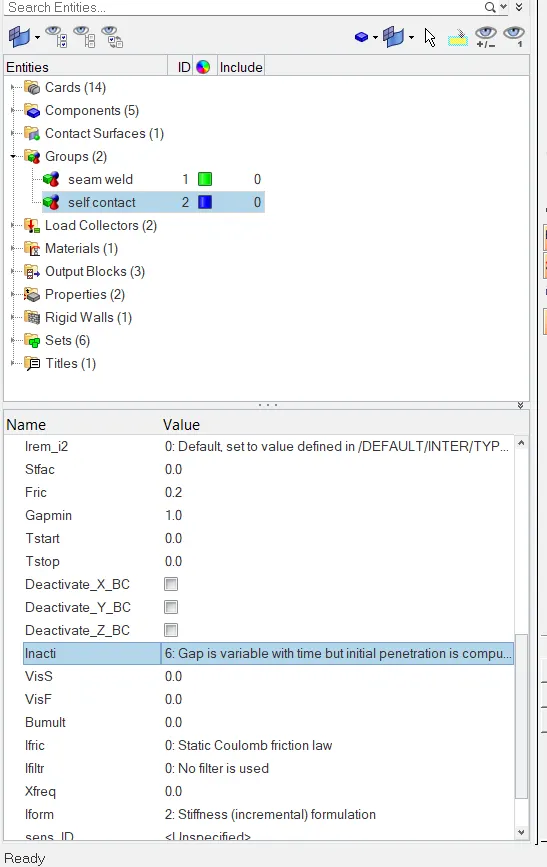
• Now, go to ANALYSIS > RADIOSS > INPUT FILE > INCLUDE CONNECTOR > OPTIONS = -NT 4 > RADIOSS.
• This will run the Radioss simulation.
• Open .out engine file from saved folder and check final value of Energy error, Mass error, Simulation time and Total no of cycles.

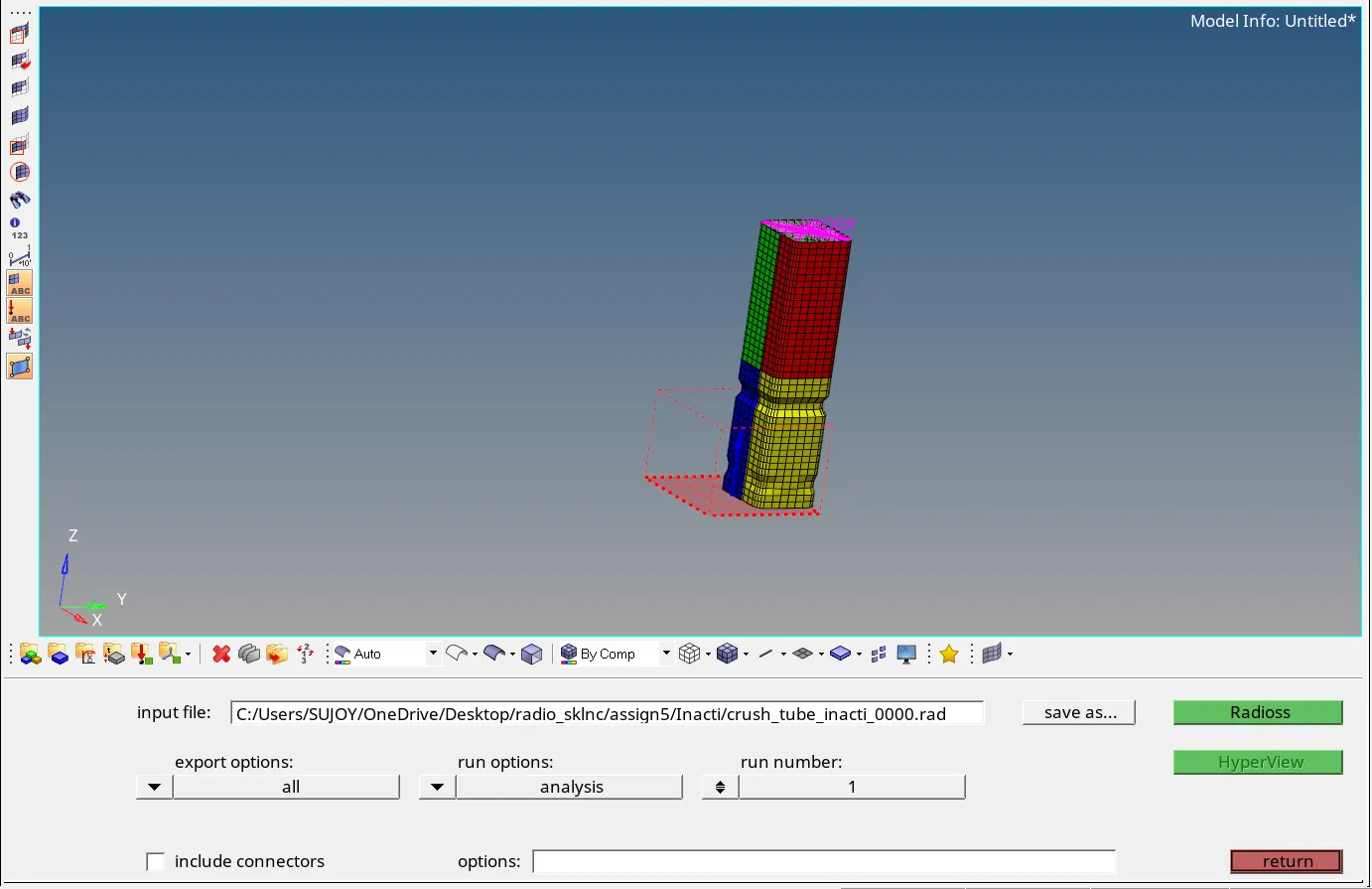
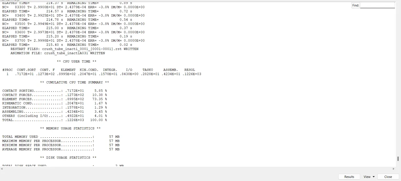
• Click on view Results, which will open Hyperview window.
• In Hyperview go to CONTOUR > RESULT TYPE > VON MISES > AVERAGING METHOD > SIMPLE > APPLY.

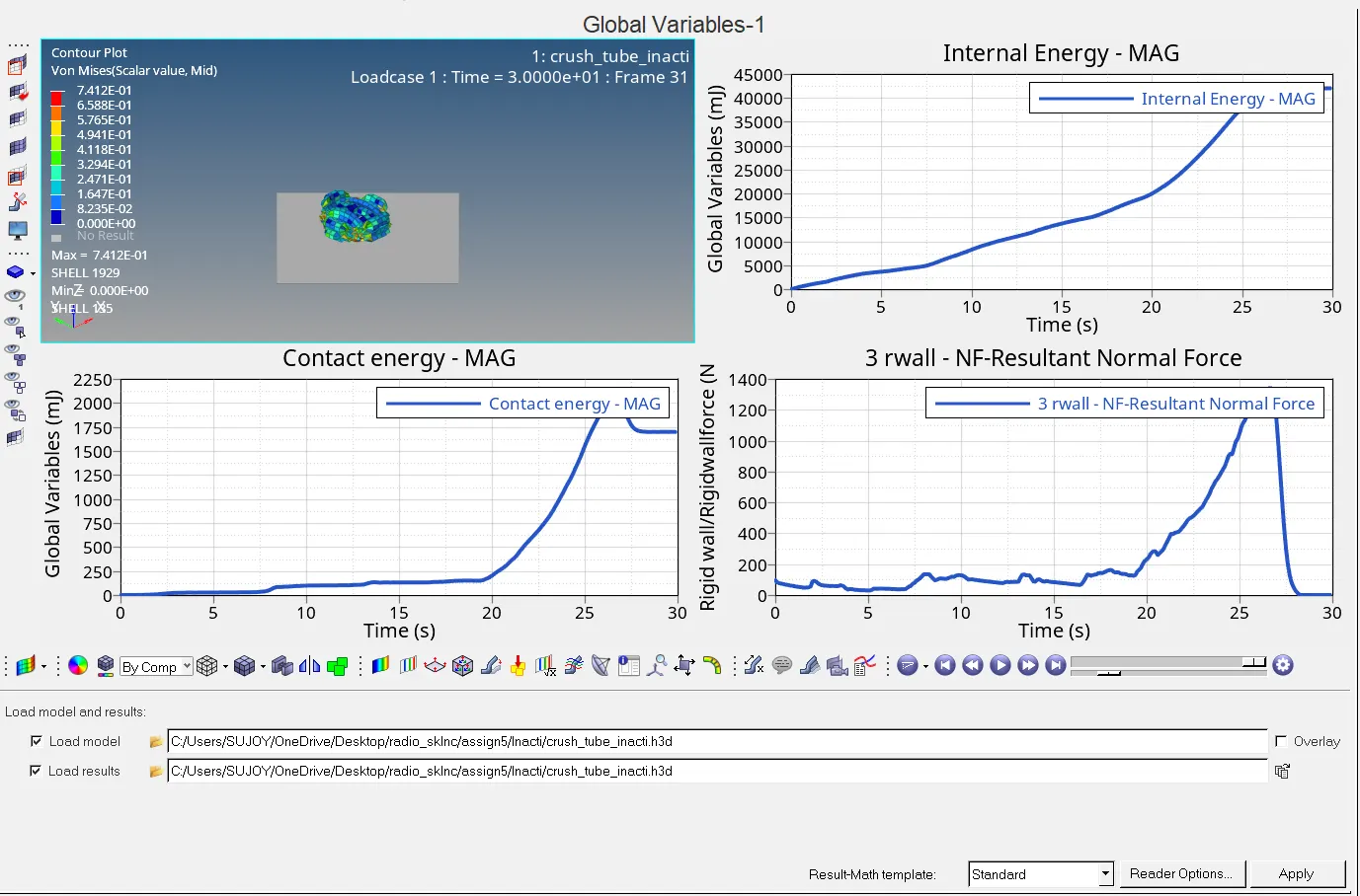
<iframe src="https://www.youtube.com/embed/MeWZqFZ8pPQ" allowfullscreen="allowfullscreen"></iframe>

• Case 3: Create the type 11 contact and run.
• Go to FILE > IMPORT > SOLVER DECK > CRUSH TUBE_0000.RAD > IMPORT.
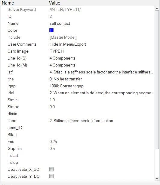
• CREATE > INTERFACE > TYPE 11 and set the following values in the card as shown in the image. Select all the 4 components for the master and slave line.

• Now, go to ANALYSIS > RADIOSS > INPUT FILE > INCLUDE CONNECTOR > OPT
• This will run the Radioss simulation.
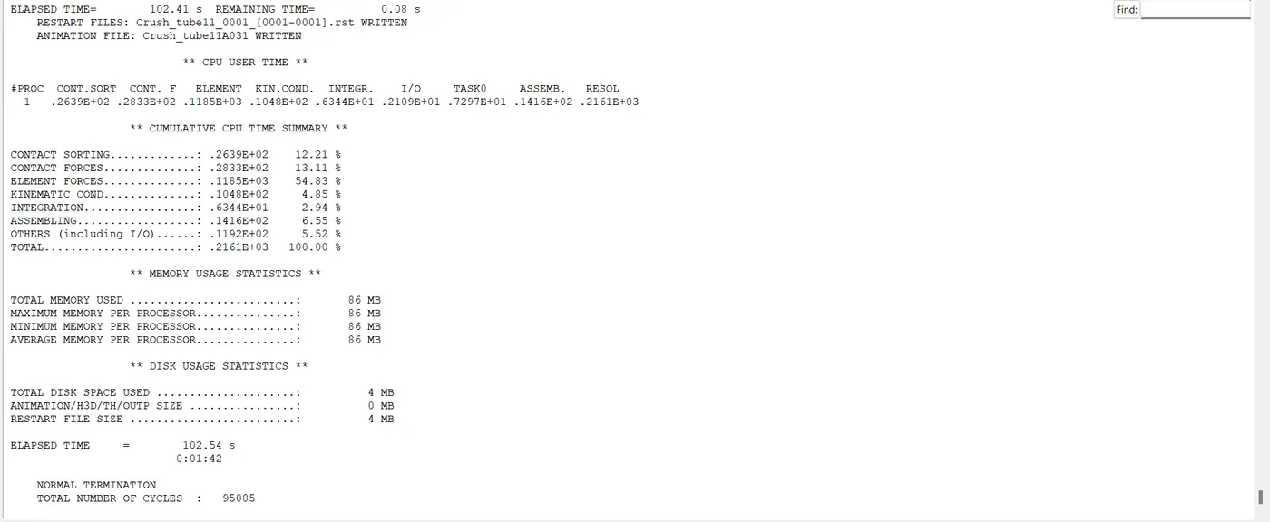
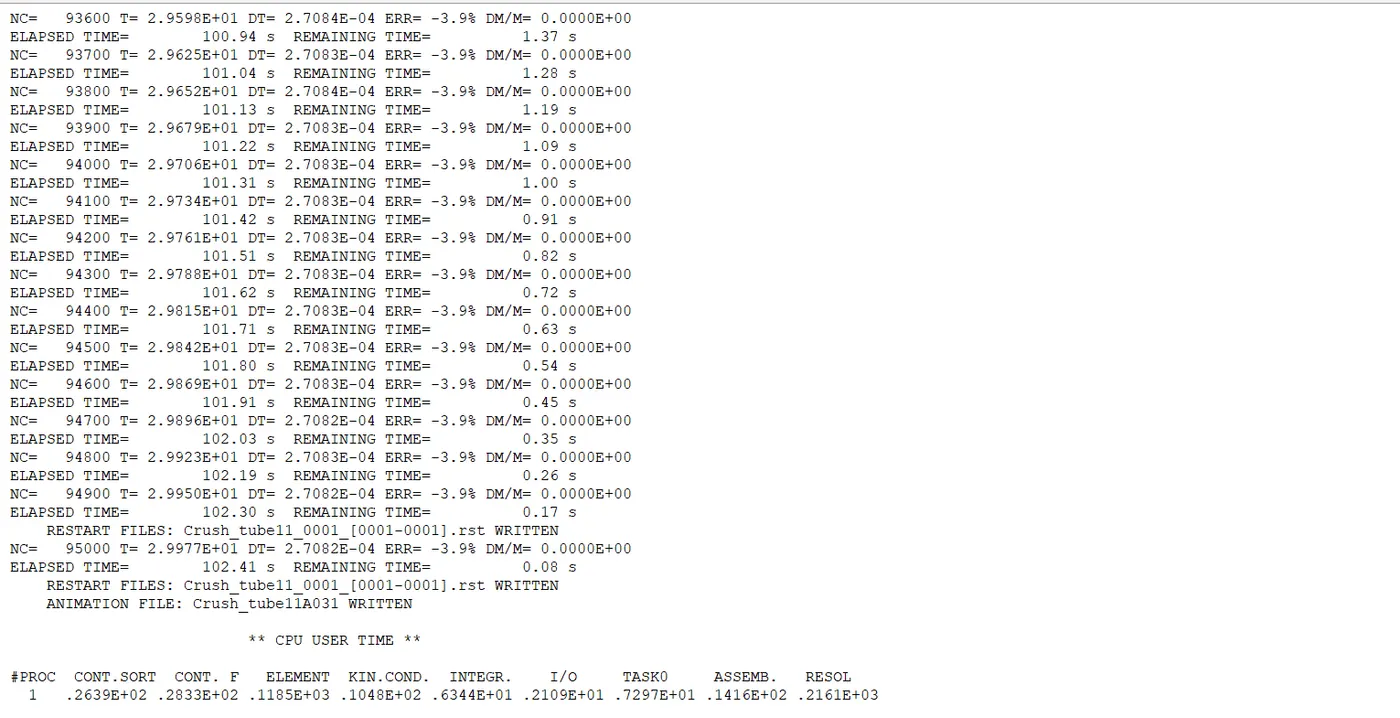
• Open .out engine file from saved folder and check final value of Energy error, Mass error, Simulation time and Total no of cycles.
• IONS = -NT 4 > RADIOSS.

• Click on view Results, which will open Hyperview window.
• In Hyperview go to CONTOUR > RESULT TYPE > VON MISES > AVERAGING METHOD > SIMPLE > APPLY.

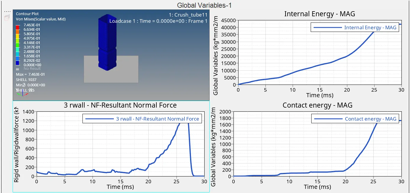
• In this case Type 11 interface is used which removes the edge to edge intersections. In the model as there are few edges the result doesnt vary with respect to the earlier results.
• Open Hypergraph 2D and load T01 file.
• There is more energy error than type 7 interface.

Case 4 :- Remove both notches  and remove boundary condition on rigid body node then run.

• In this case, the notch needs to be deleted and make it into a plane mesh.
• To delete the Notch, go to the Tools panel and select Delete option > Select the Elements to delete > Click on delete Entity.
• The Notch elements are deleted.
• To create a plane surface, go to the 2D panel, Select Ruled option > Select the first Node list > Select the Second Node List > Click Create. >> The mesh is created Give the element length as 6 > Click Recalculate > Click mesh.
• The mesh is created properly.
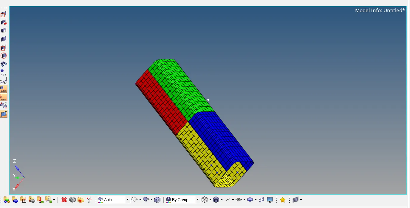
• Now to delete the Boundary conditions, go to the Solver Deck, If the Solver deck is not visible, Go to the View tab in the Standard menu bar > Click Browse > Click Hyper Mesh > Click on Solver > The Solver Deck will be opened. > Delete the BCS Entity in the Solver Deck.
• To simulate the model, go to the Analysis Panel, Select the Radioss Option > Select the area to save the file (Note: Save the File in separate folder naming Case 4 as it will be easy to check the models) > Check include collectors box > In the options tab, type “-nt 4” > Click Radioss. The Simulation is run successfully.

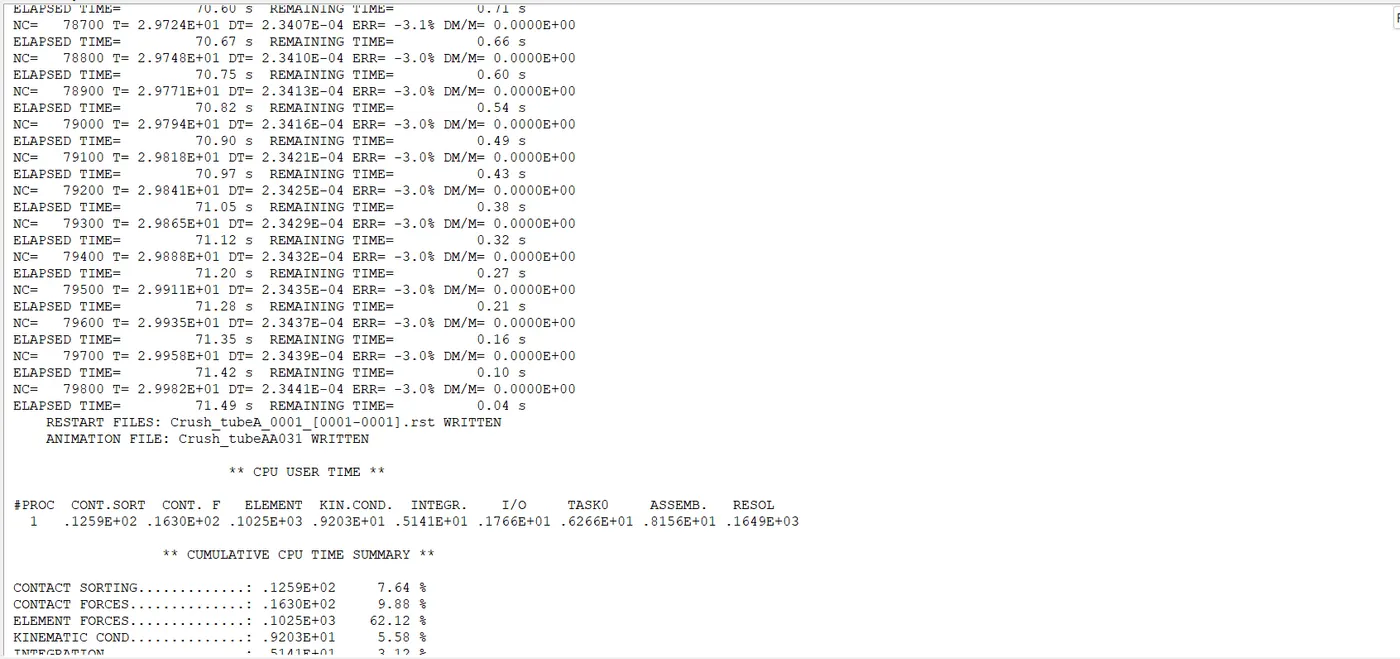
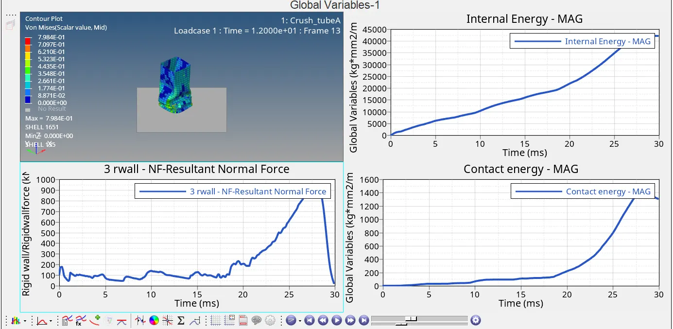
• For this simulation, the max contact force is created as 61.09 N where as the time history (TH) for all the components are created inorder to study the deformation and energy variation in each component wrt to time.
• The Internal energy for the p_shell_2.0 components is increasing at the beginning because it is attached to the rigid wall and deform smoothly there is no notch area where as the stiffness is constant over all the model. The Internal energy for the p_shell_3.0 components is zero for 10ms and linearly increasing to deform (compression takes place) at a velocity 13.3 m/s. The end of this components defines the rigidity with a translational (z-direction) degree of freedom. The Total energy for all the 4 components are varying individually with absence of boundary conditions.
• The Kinetic energy for the p_shell_2.0 components is varying at the beginning for 10ms and maintained as constant which means no more deformation occurs. Because of Notch area presents over the components it deforms very quickly. The Kinetic energy for the p_shell_3.0 components is continuously varying over the time 25ms means deformation takes place  (compression) at a velocity of 13.3 m/s. 
• The contact energy is varying at a very small amount at the beginning and there is a sudden peak formed because there is large amount of energy developed at the end of deformation. The overall elements are became overlapped or compressed which will developed large force on the rigid wall around 1200 Newton and energy created is 1.3 kJ.

• Case 5: Create a new notch in the middle ,select the whole section and run.
• Go to FILE > IMPORT > SOLVER DECK > CRUSH TUBE_0000.RAD > IMPORT.
• For this case we have to create a notch at the middle section.
• Hence, first use align option for removing all the notches and then go to TOOL > TRANSLATE option to create a notch at the middle section.

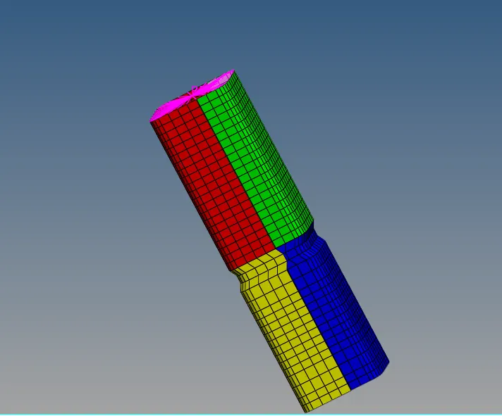
• Now, go to ANALYSIS > RADIOSS > INPUT FILE > INCLUDE CONNECTOR > OPTIO
• This will run the Radioss simulation.
• Open .out engine file from saved folder and check final value of Energy error, Mass error, Simulation time and Total no of cycles.
• NS = -NT 4 > RADIOSS.

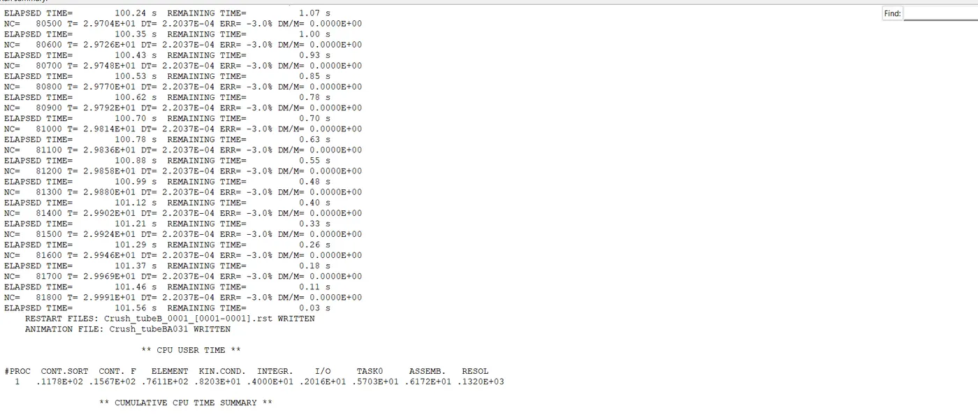
• Click on view Results, which will open Hyperview window.
• In Hyperview go to CONTOUR > RESULT TYPE > VON MISES > AVERAGING METHOD > SIMPLE > APPLY.

• Open Hypergraph 2D and load T01 file.
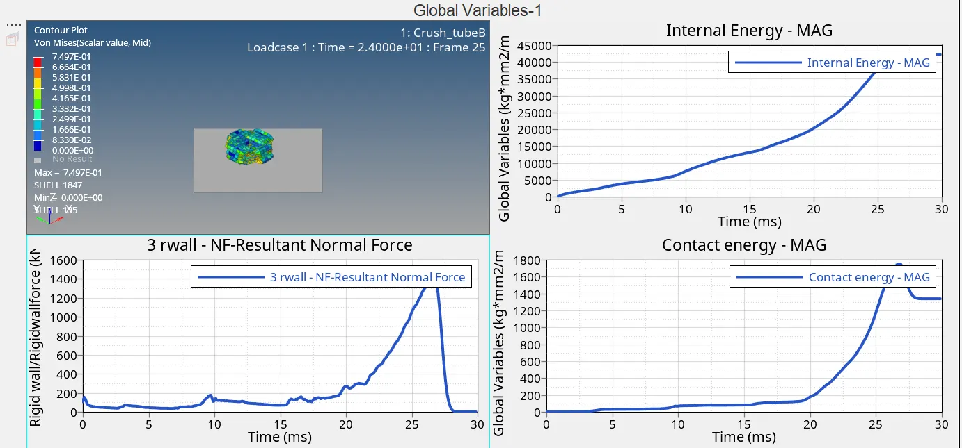
• Go to GLOBAL VARIABLES > INTERNAL ENEGRY, KINETIC ENERGY and TOTAL ENERGY > MAG > APPLY. This will plot the energy graph.
• In this graph we can observe a slight reduction in teh kinetic energy and a slight increase in the internal energy at 11ms, where the deformation in the upper section starts. This is mainly due to the notch created at the middle section of the tube.
• Go to GLOBAL VARIABLES > CONTACT ENERGY> MAG > APPLY. This will plot the energy graph.

• Case 6: Create a new notch with nodes only from opposing 2 faces and run.
• Go to FILE > IMPORT > SOLVER DECK > CRUSH TUBE_0000.RAD > IMPORT.
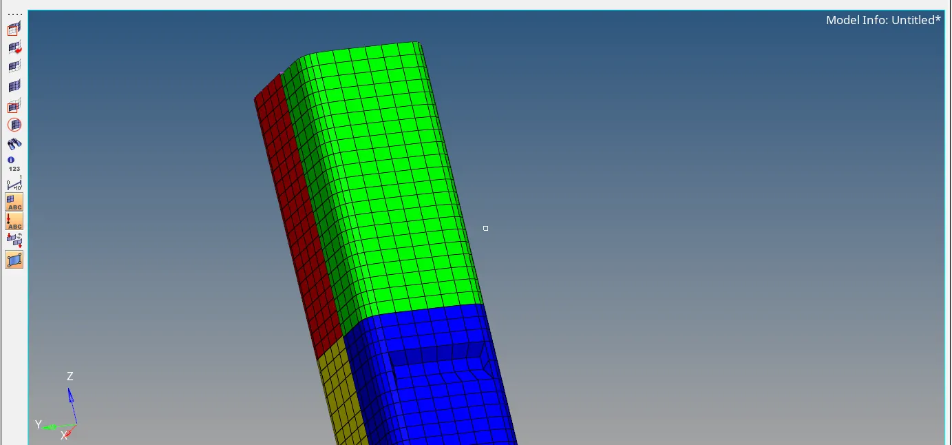
• For this case we have to create a notch with nodes only from opposite two faces.
• Hence, first use align option for removing all the notches and then go to TOOL > TRANSLATE option to create a notch on the opposite two faces.

• Now, go to ANALYSIS > RADIOSS > INPUT FILE > INCLUDE CONNECTOR > OPTIONS = -NT 4 > RADIOSS.
• This will run the Radioss simulation.
• Open .out engine file from saved folder and check final value of Energy error, Mass error, Simulation time and Total no of cycles.

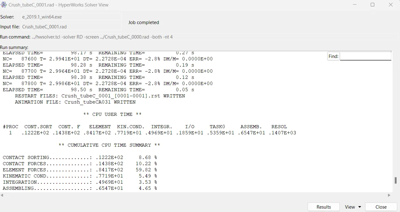
• Click on view Results, which will open Hyperview window.
• In Hyperview go to CONTOUR > RESULT TYPE > VON MISES > AVERAGING METHOD > SIMPLE > APPLY.

• n this case the initial deformation is again at the notch section due to the stress concentration. But the faces having the notch deform inwards and the faces with no notch deform outward.
• Open Hypergraph 2D and load T01 file.
• Go to GLOBAL VARIABLES > INTERNAL ENEGRY, KINETIC ENERGY and TOTAL ENERGY > MAG > APPLY. This will plot the energy graph.
• As compared to the previous cases the graph does not show slight deformation at 11ms.
• Go to GLOBAL VARIABLES > CONTACT ENERGY> MAG > APPLY. This will plot the energy graph.
• The contact energy recorded is lower than the previous cases. The contact energy at the end is about 1500 kgmm2/ms2. The increase in the contact energy at the beginning is very less.
• Go to GLOBAL VARIABLES > RWALL > NORMAL RESULTANT, TANGENT AND TOTAL FORCES > APPLY. This will plot the rigid wall forces.

• Here type 7 interface is used for the first two cases and then the type 11 contact is created. Hence. both the interface work together making the simulation stable. The deformation of the tube is observed to be in layers, where the slave nodes try to enter the master gap, the penalty method creates a spring and resistive forces are applied. The energy error is caused when the stiffness value increases to a greater value, minimizing the time step and hence the elements are deleted. The deletion of the elements releases the energy.
• In the second case, we only observe the change in simulation time, because the Inacti6 is set which performs initial penetration checks before the simulation.
• In the third case the type 7 and type 11 interface work together increasing the simulation time. The energy error is also increased.
• In the fourth case. we observe less no of cycles and lower energy error as the boundary conditions and the notches are removed.
• In the fifth case, we observe the increase in the energy error due to the notch created at the middle section here the four components are closer to each other when deformed.
• In sixth case, we observe the no of cycles to be the greatest among all the cases. Also there is reduction in the energy error as opposite face notch is created. 

  LEARNING OUTCOMES:

  • To apply the different interfaces for the components.
  • To study the results of the interface types.
  • To understand the parameter checks before simulation and during simulation.
  • The significance of Inacti 6.
  • To plot the energy and the rigid wall forces.

   

  CONCLUSION:

  • Hence, by performing this project we conclude that the we have studied the type 7 and type 11 interface and also their working together. We also studied the effect of notches based upon their location and no of notches. The parameters checked before the simulation and during the simulation are also studied.

•