Assignment 4-RADIOSS Material Laws Challenge
AIM:
To run crash analysis on the given model by applying different materials laws available in Radioss and post-process the results
Objective:
To carry out simulations of the given starter files and compare the results. There shall be 7 cases (according to given parameters) and they are to be compared primarily via animations and plots. The files to be worked on are the FAILURE JOHNSON_0000.rad file and the LAW27_0000.rad file. The cases are as follows:
1. Law 2 (file: FAILURE_JOHNSON 0000.rad) - base simulation.
2. Law 2 (file: FAILURE JOHNSON 0000.rad) with Ifail_sh=1, Dadv = 1, and Ixfem = 1.
3. Law 2 (file: starter file for case 2) with fail/JOHNSON card deleted. 4. Law 2 (file: starter file for case 3) with EPS_p_max value deleted
5. Law 1 (file: FAILURE JOHNSON_0000.rad) with fail/JOHNSON card deleted and values for density. E, nu assigned
6. Law 27 (file: LAW27_0000.rad) with recommended shell properties.
7. Law 36 (file: LAW27_0000.rad) with recommended shell properties and given reference curve.
Procedure:
CASE 1
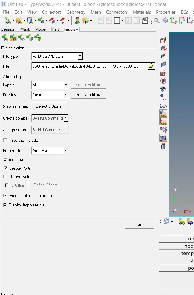
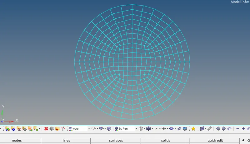
1. With Hyperworks open, the file is imported via the 'import solver deck' option through File> Import. The 'FAILURE_JOHNSON_0000.rad file is selected and import' is clicked
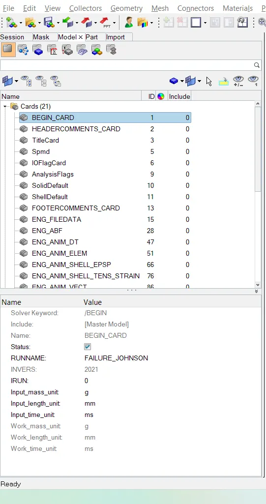
Then in the solver browser some cards are verified, inorder to have clarity on some aspects. Among them, the first card to be checked is "Begin card". Inorder to check for the unit system. The unit system plays a prominent role for assigning all of the values. The unit system for this appears as shown in fig
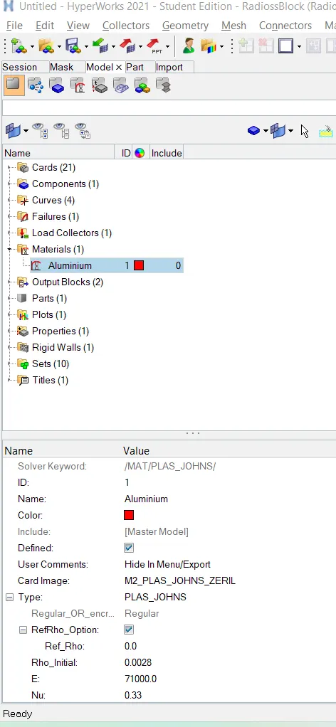
The material card is the next card to be verified, inorder to see the properties assigned to the material. The material card appears as shown
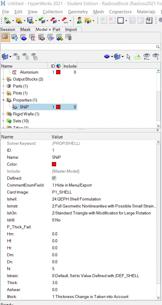
Next card to be verified is property card. In property card, the properties assigned to the given material is seen. The property card with the assigned parameters appears as shown in fig. below
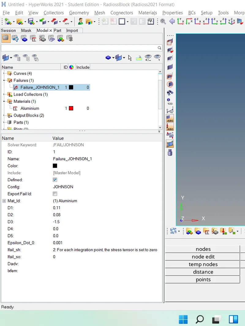
2. For this case, we are to run the simulation as is. The file has the following material and failure cards:
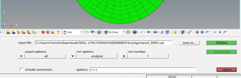
To run the simulation, we go to Analysis > Radioss from the bottom panel. We then need to save the file. The file is saved as "assignment4_0000.rad. After saving, we can go ahead and check the include connectors' box and type in ¹-nt 4' in the options text box, before clicking 'Radioss'.
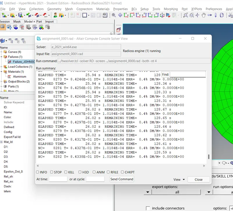
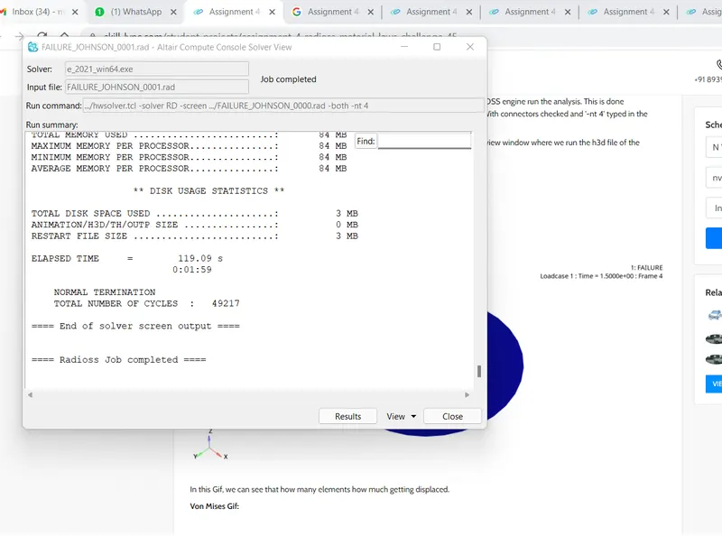
On clicking 'Radioss, we get the solver window, which basically tells us what the RADIOSS solver is doing. After a few minutes, it lets us know that the file has been processed.
3. Once the simulation is complete, now we just need to visualize it. For that, we need to switch to the Hyperview utility. This can be done by clicking the client selector option in the toolbar (might need to be activated from View> Toolbars > Hyperworks > Client Selector). In that menu, we can select Hyperview to switch to it.
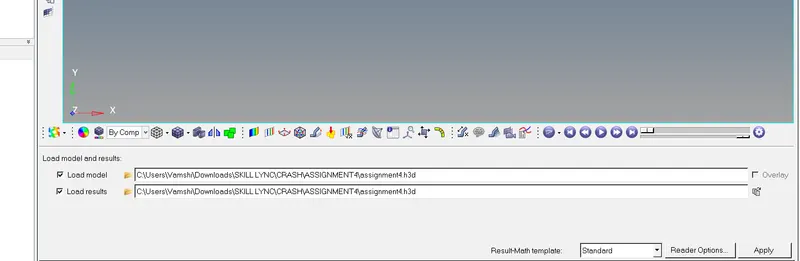
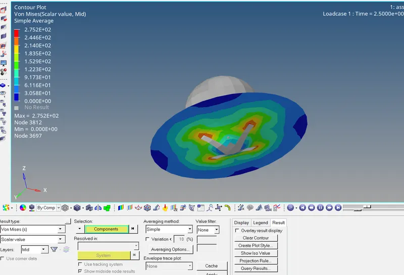
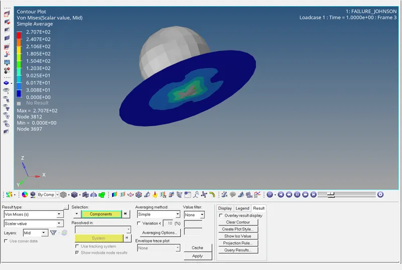
4.After accessing Hyperview, we are asked to input the simulation file. For this, we shall be using the h3d file that was generated when RADIOSS processed the starter file . It should be generated in the same folder. After selecting it, we can click 'apply. Doing so generates the simulation animation. We can change what is being represented by selecting the 'contour' option in the toolbar. In this case, we can change the result type to 'Von Mises' and change the averaging method to simple. Doing so creates the Von Mises stress contours as shown:
4. Next step is to carry out energy error and mass error checks and this is done by analyzing the RADIOSS engine output file. This can be accessed from the same directory as the starter and engine files and is denoted by the 'out' extension. We need to check the file that contains_0001.out' by using any text editor.
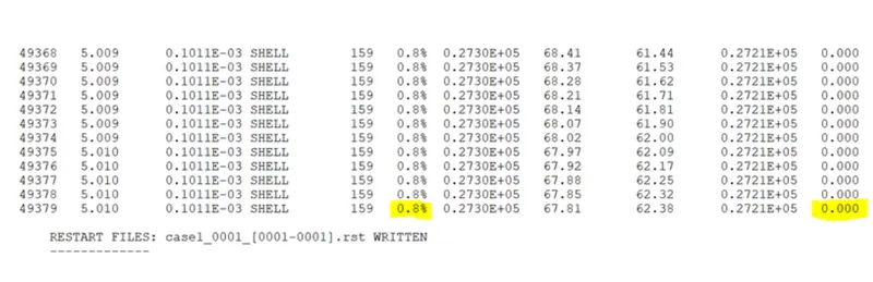
On opening the file and scrolling down to the end, we can see the final energy and mass error values.
The final energy error is 0.8%, which is very acceptable. The closer to O it is, the better. Added, there is no mass error. Overall, these are very good values.
5. Now we can plot the graphs. For this, we shall be using the Hypergraph client. We can switch to it using the same client selector option in the toolbar.
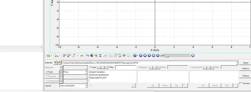
In the Hypergraph section, we are met with a graph and in the panel below, we are to input a file. For this, we will be using the result file generated by the RADIOSS solver (also known as the 'TO1 file). This file is available in the same directory as the starter, engine and animation files. The file name ends with TO1.
After adding it, we can select the variables that would go with time (x-axis).
CASE 2
1. The process is repeated with slight changes. Just as last time we import 'assignment4_0000.rad' via the solver deck import process.
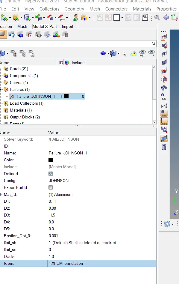
2. This time, we make some changes to the fail/JOHNSON card. It can be accessed via the model tab, under the 'Failures' submenu.
On clicking Failure_JOHNSON 1, we can edit attributes of the card in the entity editor window in the bottom left. We are looking for the Ifail_sh, Dadv, and Ixfem attributes in particular.
The following values are assigned: Ifail_sh=1, Dadv = 1, and Ixfem = 1
3. After the values are changed, we continue as in the previous case by letting the RADIOSS engine run the analysis. This is done via Analysis > Radioss. This time, the file is saved as 'FAILURE_JOHNSON_0000.rad. With connectors checked and '-nt 4' typed in the options box, we can click the Radioss button to run the analysis.
4. After the solver window completes the analysis, as usual, we can switch to the Hyperview window where we run the h3d file of the current analysis - .h3d and set the Von Mises stress contours:
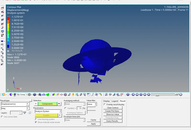
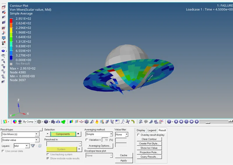
From both simulations, we can see that the elements are getting crack when they are failing. Elements are not flying away in this case. So when the elements break beyond the limit it gets deleted. But those elements are very few.
5. After that, we can go ahead and check the energy and mass error on the RADIOSS output file,
CASE 3
1. Again, we need to switch to Hyperworks and import the solver deck file for this case and that would be 'FAILURE_JOHNSON_0000.rad., the starter file created in the previous case.
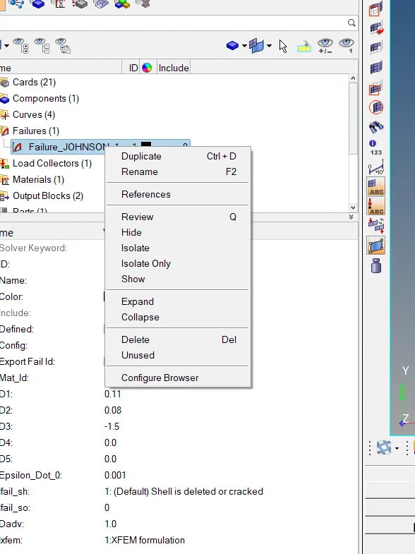
2. As we did in the previous case, we need to make changes to this file as well. We need to switch to the model tab and this time, we will be deleting the fail/JOHNSON card altogether. To do that, we can go to Failures > Failure_JOHNSON 1. Right-click Failure JOHNSON_1 and select 'delete.
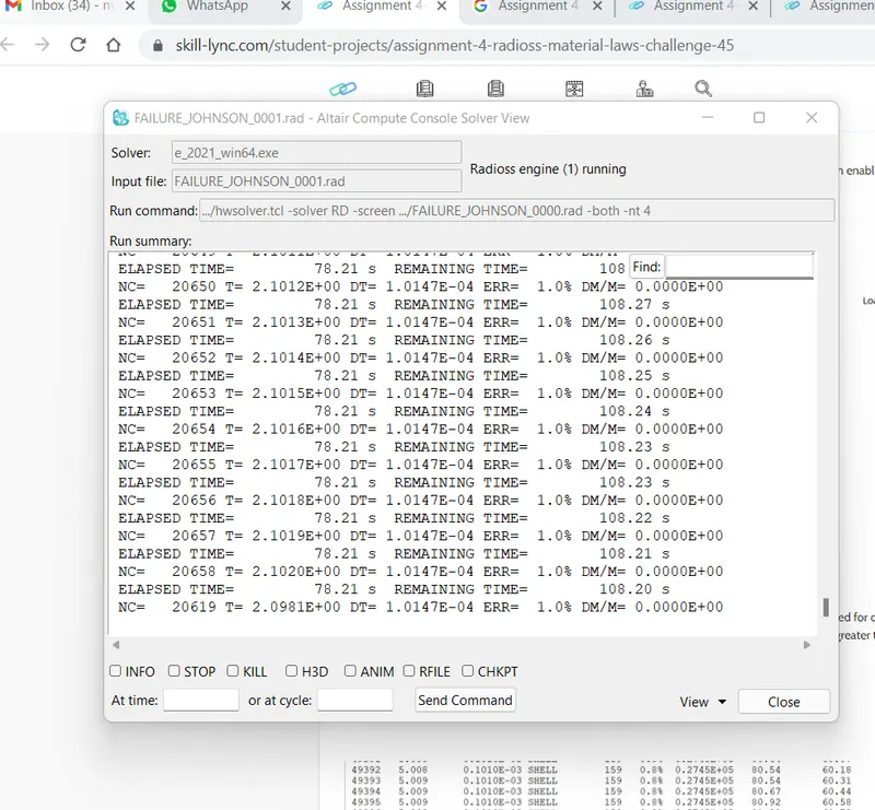
3. After deleting, we are to run the RADIOSS analysis as we did in previous cases through Analysis > Radioss. We can save the file as 'FAILURE_JOHNSON_0000.rad., enable connectors, type '-nt 4' in the options box and click 'Radioss' to run the analysis. After the Radioss solver is complete, we can switch to Hyperview.
4. On Hyperview, we can load the h3d file (Law2_epsmax_nofail.h3d) and click 'apply. We can then enable the Von Mises contouring and view the simulation.
The energy error is very close to O and the mass error is non-existent. Now we can switch to Hypergraph to plot the graphs. They shall be
analyzed in the next section.
CASE 4
1. We can switch back to Hyperworks and work on the next case. We shall import the case 3 starter file-'FAILURE_JOHNSON_0000.rad.
2. This time, we are to delete the EPS_p_max value. Going to the model tab, we can go to Materials > Aluminium. In the entity editor window, we can clear the EPS_p_max value
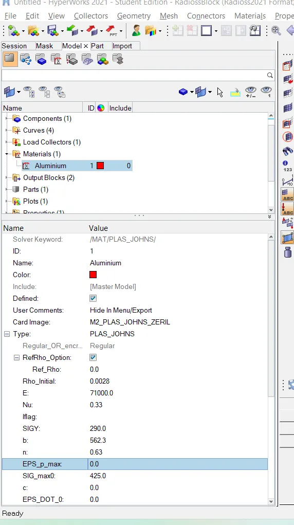
3. After that, we can switch to the Radioss analysis section via Analysis > Radioss, save the file as ''FAILURE_JOHNSON_0000.rad., enable connectors and type in '-nt 4' in the options section and run the analysis by clicking Radioss!
4. After the solver finishes its analysis, we can switch to Hyperview, run Law2.h3d, activate the Von Mises contours and view the simulation:
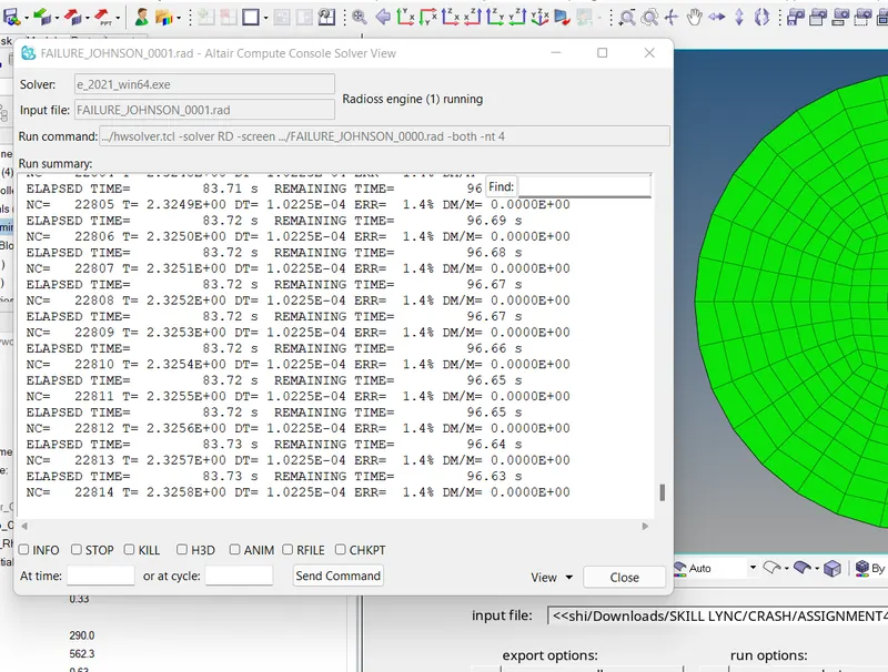
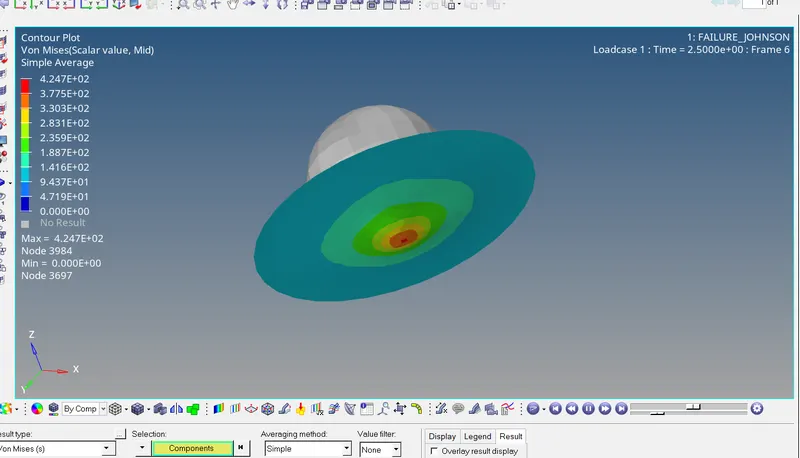
The energy error is less than 5% and mass error is non-existent. We can now switch to Hypergraph to plot the graphs for this simulation.
CASE 5
1. We repeat the process again but this time, we import the main starter file - FAILURE JOHNSON 0000.rad. As in case 2, we can delete the fail/JOHNSON card via the model tab.
2. After that, we can move to Materials > Aluminium. In the entity editor window, we can change the card image to M1 ELAST, which is Law 1.
After doing that, we can set the values for Rho_Initial, E & Nu as follows: Rho_initial=0.0028, E- 71000.00, nu-0.33.
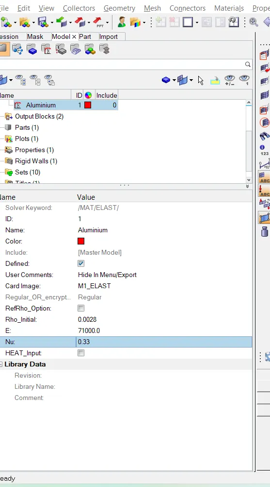
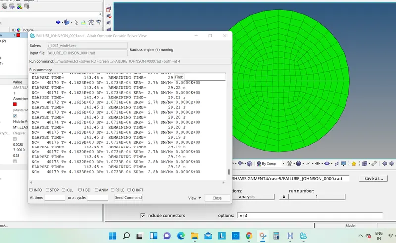
3. Now we can switch to Analysis > Radioss and save the file as 'Law1_0000.rad. Just as before, we can enable connectors and type '-nt 4' in the options box. Then, we can click radioss and let the solver run the analysis.
4. After the solver completes the analysis, we can switch to Hyperview, import the '.h3d file, enable the Von Mises contours and view the simulation
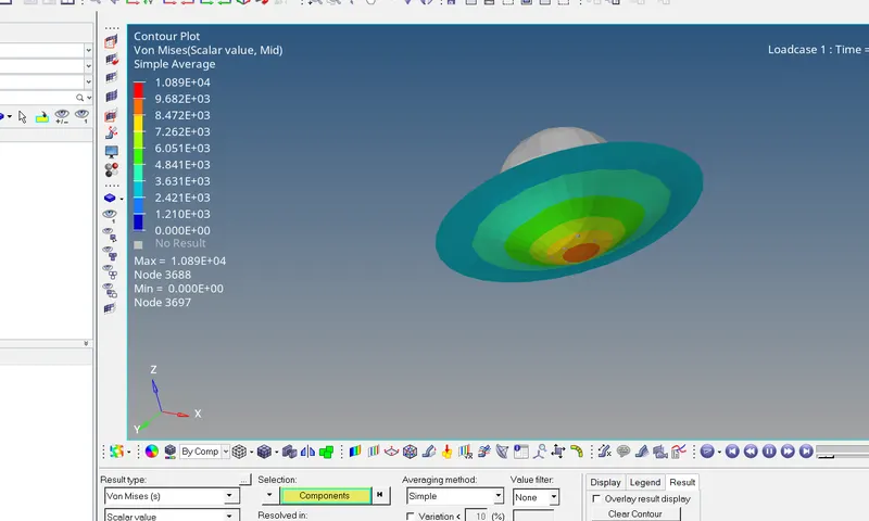
The energy error is less than 5% and the mass error is non-existent. We can then switch to Hypergraph to plot the graphs for this simulation.
CASE 6
1. We repeat the process again but this time, we import the main starter file - FROM case5
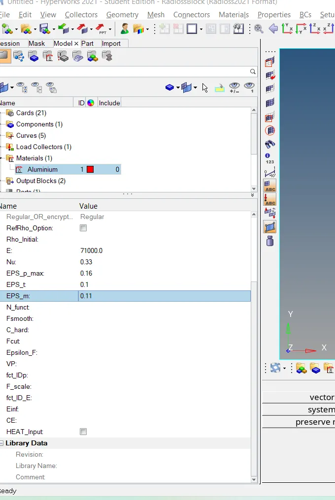
2. After that, we can move to Materials > Aluminium. In the entity editor window, we can change the card image to M36_PLAST_TAB which is Law
After doing that, we can set the values for
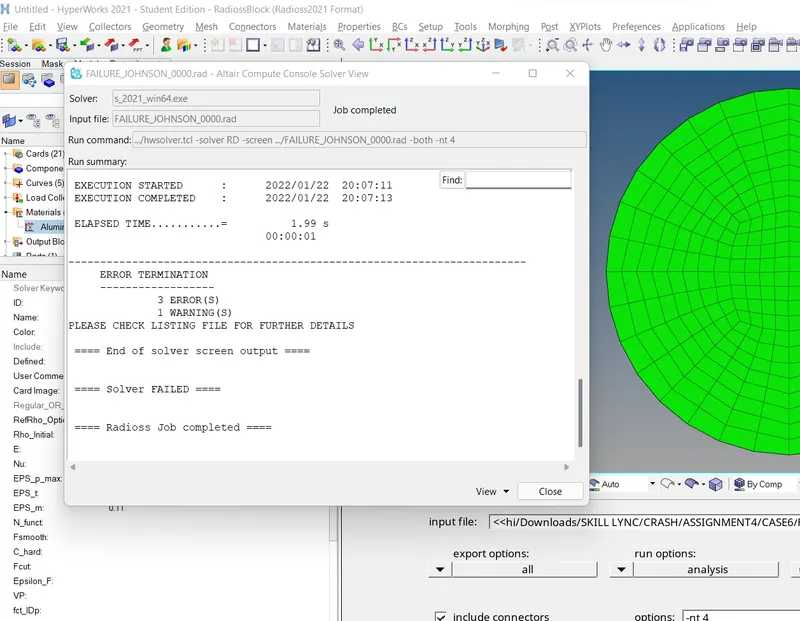
3. Now we can switch to Analysis > Radioss and save the file as 'Law1_0000.rad. Just as before, we can enable connectors and type '-nt 4' in the options box. Then, we can click radioss and let the solver run the analysis.
CASE 7
1. We repeat the process again but this time, we import the main starter file -LAW27_0000.Rad
and edit the material aluminium values as follows
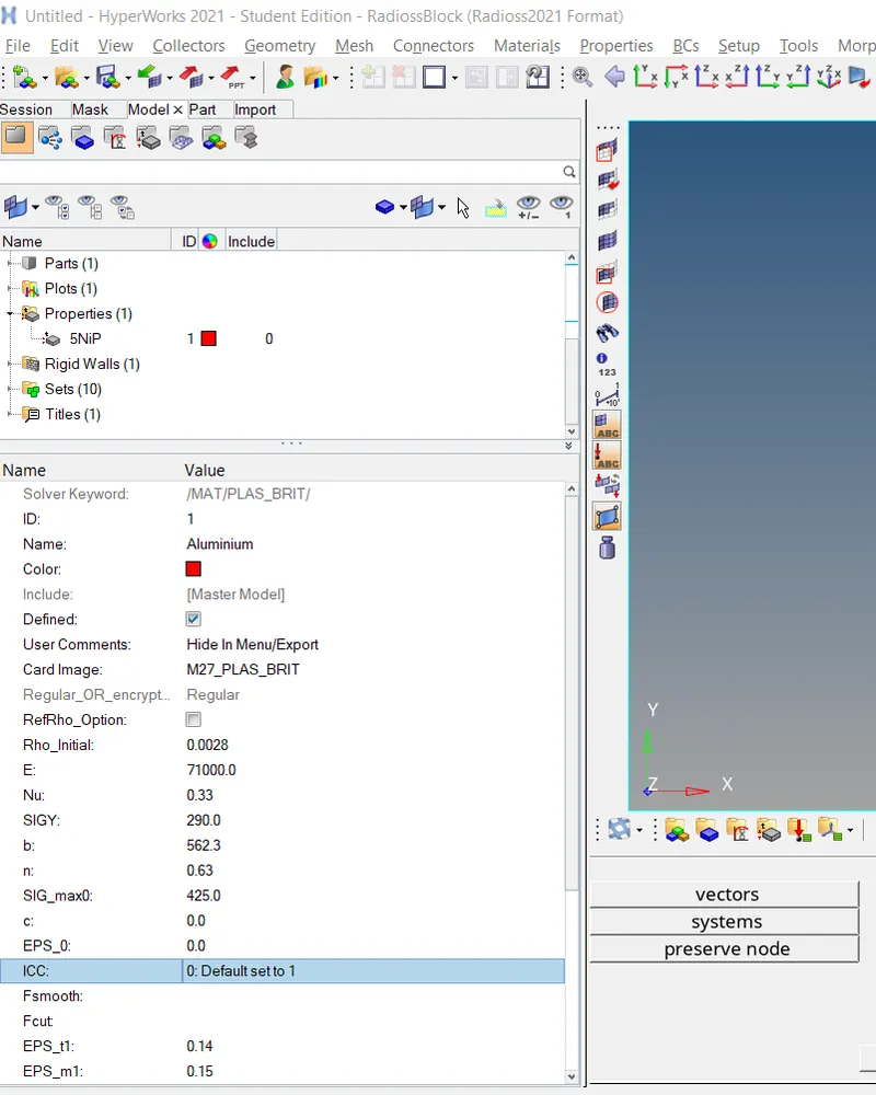
3. Now we can switch to Analysis > Radioss and save the file as law27. Just as before, we can enable connectors and type '-nt 4' in the options box. Then, we can click radioss and let the solver run the analysis.
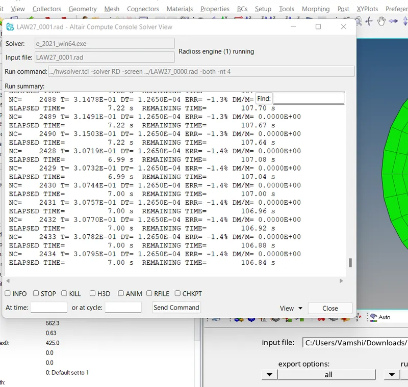
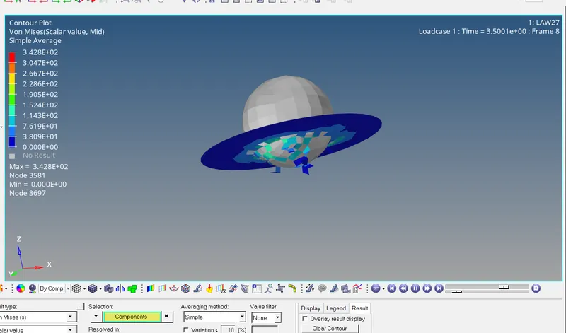
4. After the solver completes the analysis, we can switch to Hyperview, import the 'Law27.h3d file, enable the Von Mises contours and view the simulation
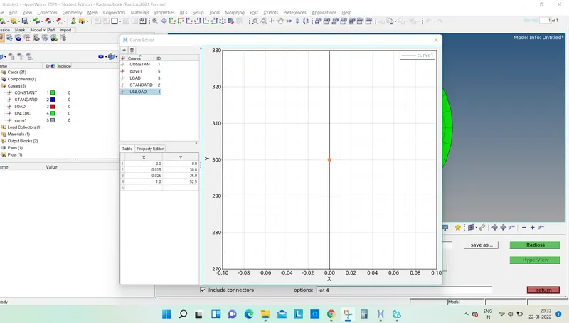
1. Switching back to Hyperworks, we can import LAW27_0000.rad again. We shall be editing certain attributes in this case.
2. Go to the model tab and here, we shall be creating a new curve (as per instructions given in the Materials 7' video). Right-Click-Create>
OBSERVATIONS
CASE 1
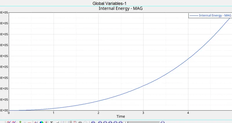
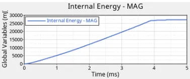
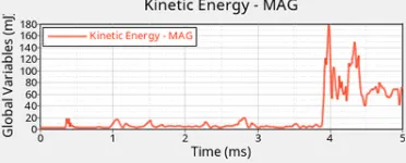
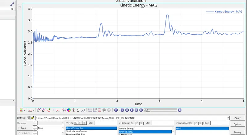
Internal energy as well as rigid wall forces are reactions to the force generated by the sphere on the sheet. Energy increases linearly until a large number of elements are deleted at around the 4ms threshold. This probably creates some vibrations and that results in a surge of kinetic energy at the same point.
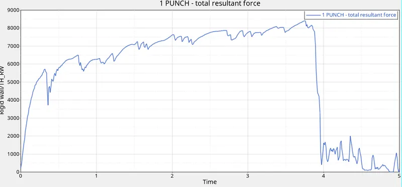
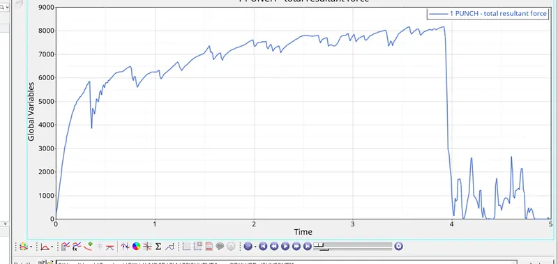
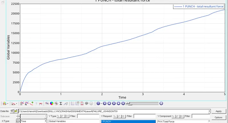
The rigid wall forces fluctuate due to element deletions and when a large chunk of elements are deleted at 4ms, the graph drops, meaning there aren't many elements opposing the force of the sphere. Most of the elements in its path have been deleted at that point
CASE 2
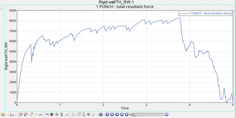
It can be noticed that in both case 1 and 2, the internal energy graphs are almost similar. They differ when it comes to the timestamp at which they plateau and this is probably due to crack propagation being a big factor
CASE3
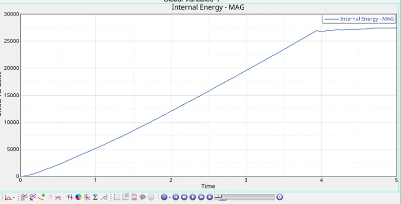
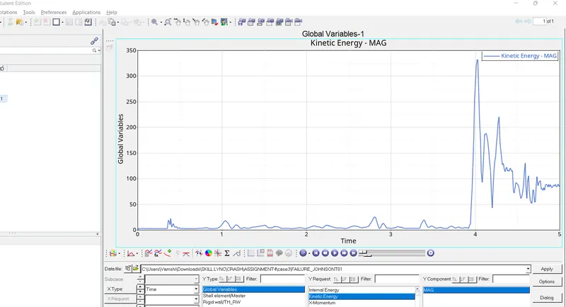
There is a linear increase in internal and total energy until a bulk of the elements are deleted from the model. This is expected since the energy absorbed by these elements go to waste due to their deletion.
This also explains the sudden drop in rigid wall forces at the same timestamp due to most elements that were in contact with the sphere during collision being deleted. The rigid wall force is basically a measure of the opposing force generated by the metal sheet against the sphere. Fluctuations occur when elements are deleted. When there are no elements to oppose the incoming sphere, there won't be any rigid wall forces.
There is a linear increase in internal and total energy until a bulk of the elements are deleted from the model. This is expected since the energy absorbed by these elements go to waste due to their deletion.
This also explains the sudden drop in rigid wall forces at the same timestamp due to most elements that were in contact with the sphere during collision being deleted. The rigid wall force is basically a measure of the opposing force generated by the metal sheet against the sphere. Fluctuations occur when elements are deleted. When there are no elements to oppose the incoming sphere, there won't be any rigid wall forces.
CASE 4
CASE 5