To study the variation of simulation results with different parameters in a simple crash scenario
Objective: To compare the simulation results with base properties and improved shell element properties
Procedure:
A. Preparing the Engine output file:
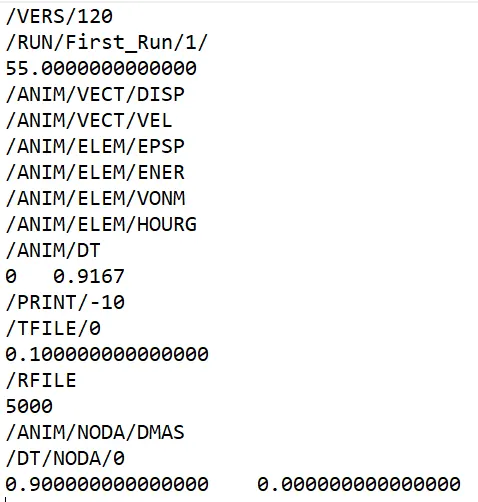
Open the Egine input file and change the Run time to 55.
For 55ms runtime and a max animation steps of 60, we get animation frequency as 0.9167 ms. We input these values in the file as shown.
B. Case 1:
1. Open the Starter input deck in Hyperworks. Go to Analysis-Radioss. Save the analysis as Case1 in a separate folder and Run it.
2. Open the Engine output file in notepad, and check the Energy and mass errors.
In this case we can see that the energy error is decreasing from 0% to -11%, which is good.
The mass error is 0.0001695
3. Open the result file in Hyperview. Animate the Displacement result and note the max displacement:
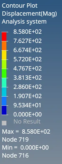
Thus max displacement is 858 mm
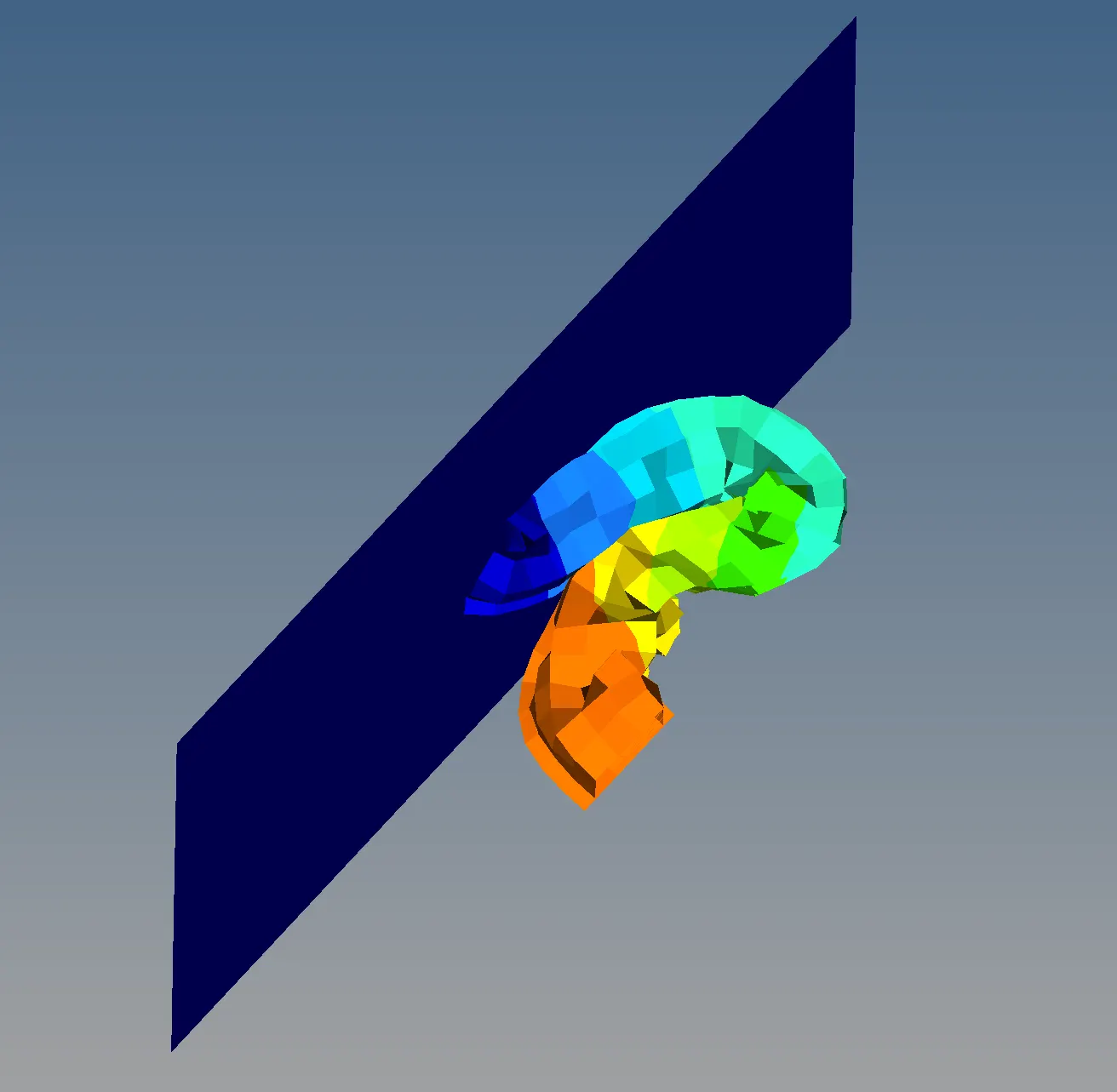
The bending behaviour is as shown:
4. In Hypergraph plot the required properties against time
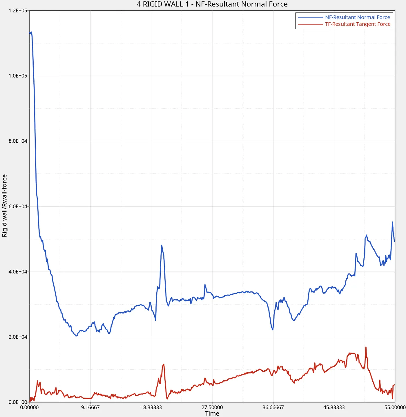
Rigid wall forces:
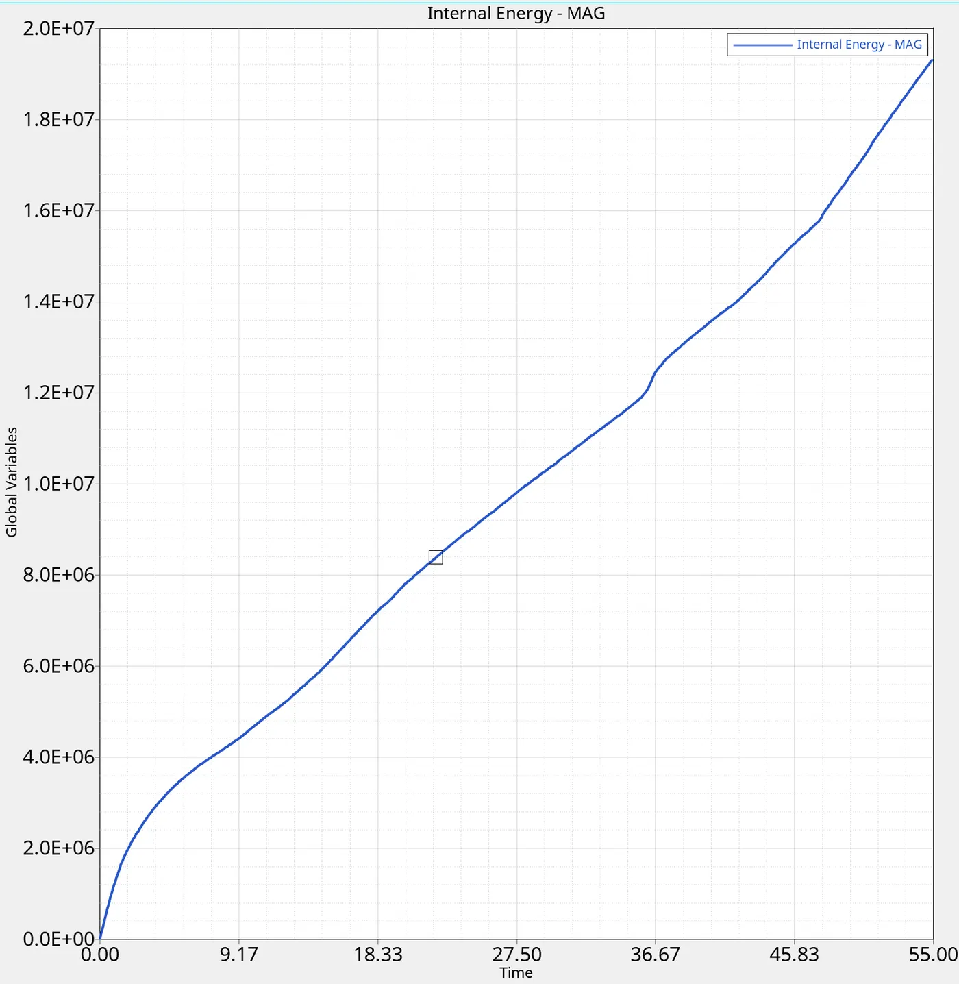
Internal Energy:
Hourglass Energy:
Contact Energy:
Total Energy:
C. Case 2:
1. The shell element property cards are changed to the recomended values as given
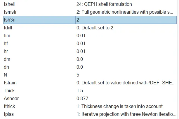
The analysis is run with a different name.
2. The Engine output file is opened in notepad and the Energy and mass errors are checked.
The Energy error decreases from 0% to -0.1%, which is good. The mass error is 0.0001695Kg
3. The simulation results are opened in Hyperview.
The displacement plot is as shown:
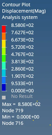
We can see that the max. displacement is 858m.
The deformation behaviour is as shown:
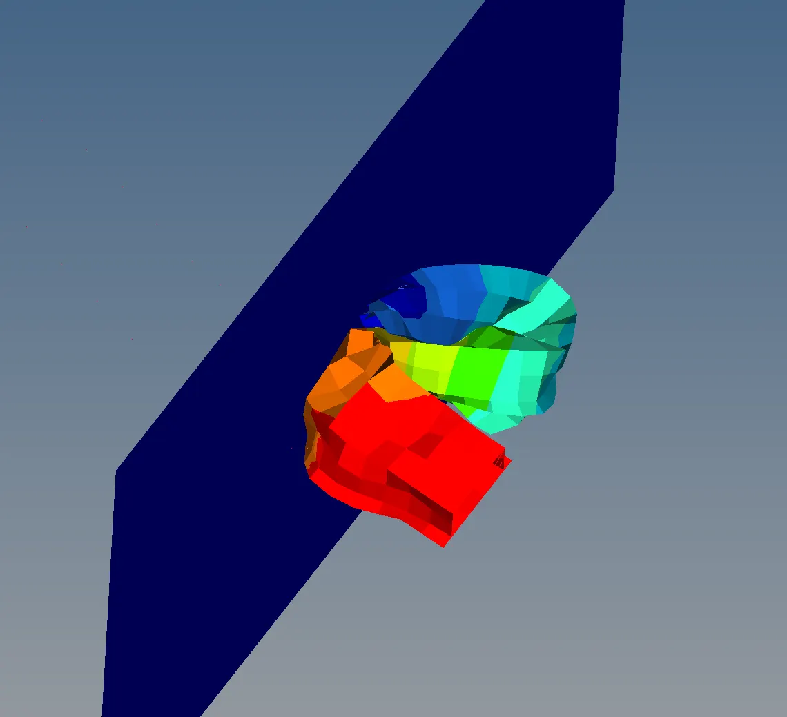
4. The rest of the values are plotted in Hypergraph:
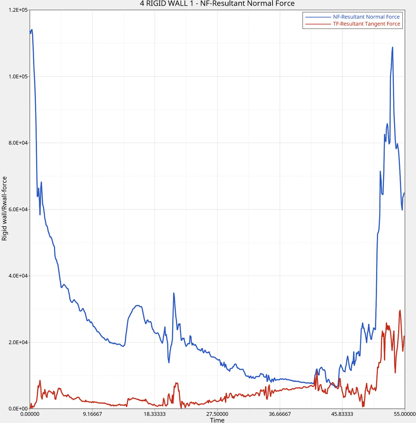
Rigid wall forces:
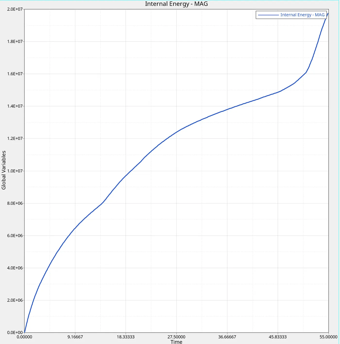
Internal Energy:
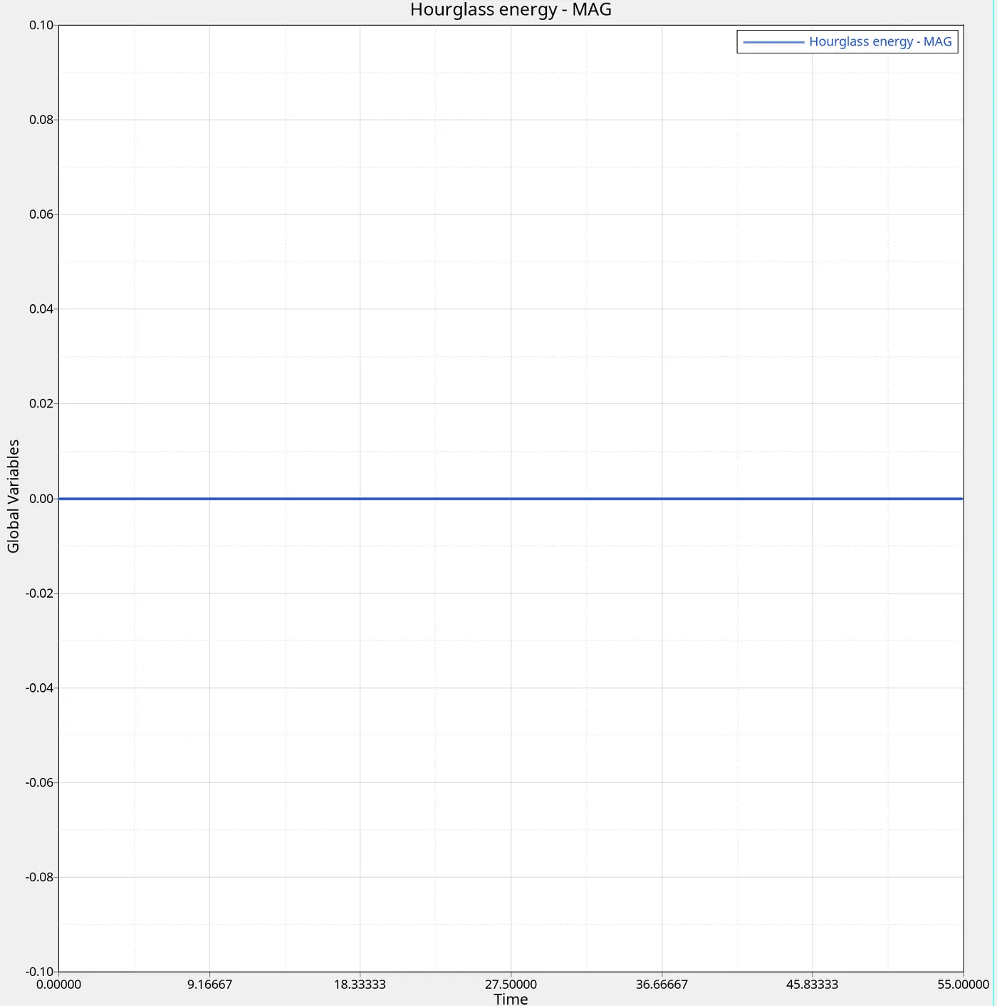
Hourglass Energy:
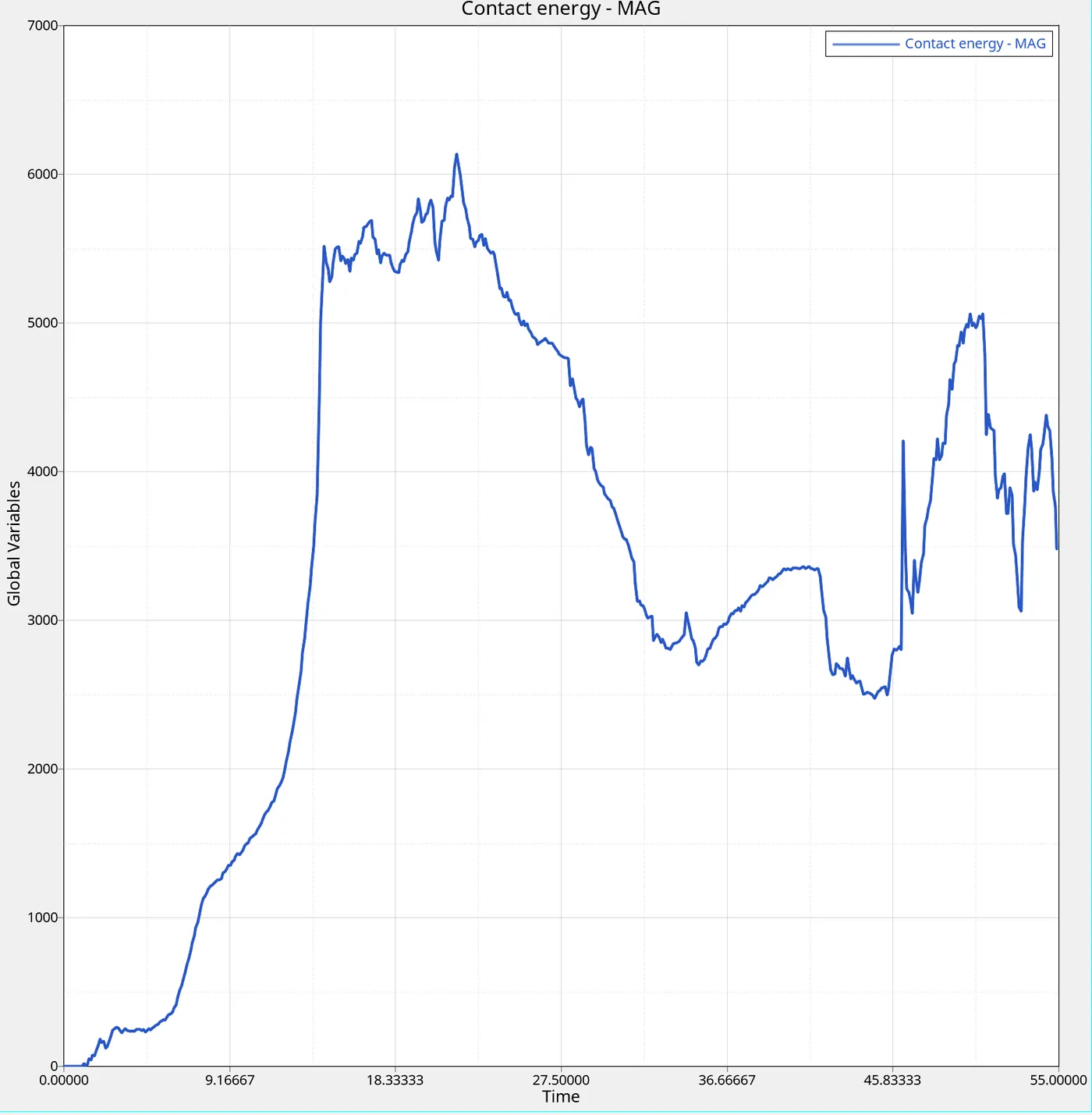
Contact Energy:
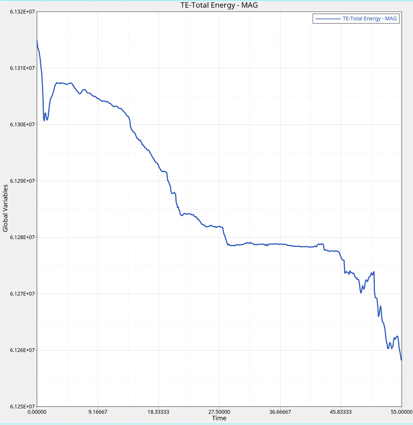
Total Energy:
D. Summary
From the above graphs we can see that the results vary substantially between the two cases. We can summarise the differences as follows:
1. In the second case the Energy error has decreased by a large value, while the mass error has stayed the same.
2. The max displacement is same in both cases, i.e 858 mm
3. Rigid wall forces in case 2 register a steep spike around 50ms, which is not the case in the first case. This indicates the deformation is significantly different in both the cases, as evident from the deformation plots too. In below plot and graph we can see the spikes just as another bend touches the rigid wall in Case 2.
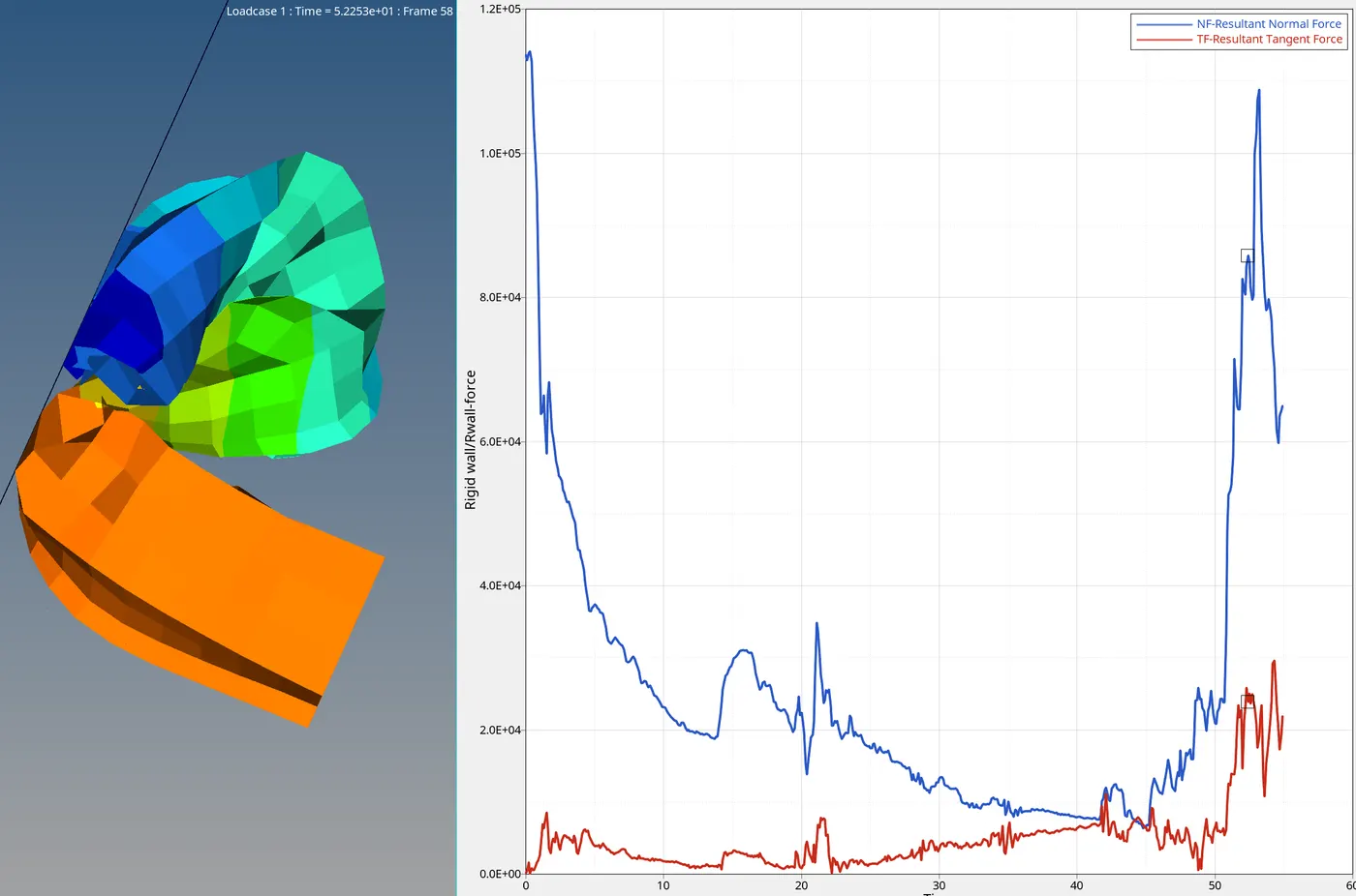
4. Internal energy in Case 1 increases fairly linearly, while in Case 2, the slope is steeper at the point of impact of the second bend with the rigid wall, and it corresponds to the increased Rigid wall forces.
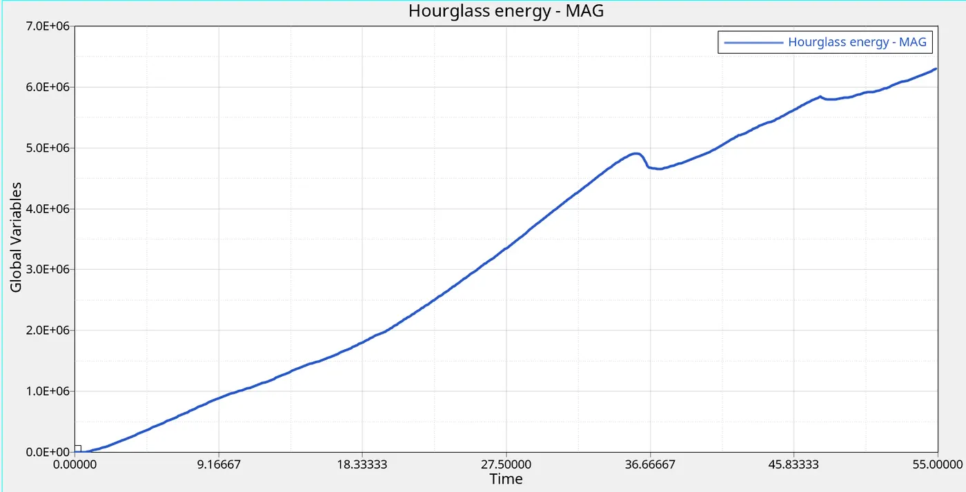
5. In Case 1 there is a substantial amount of Hourglass energy, which increases with time. Which indicates there is large amounts of hourglassing happening. This is due to the default Shell element formulation flag of 1, which utilises perturbation hourglass stabilisation, which is inefficient compared to physical hourglass stabilisation.
There is no Hourglassing in Case 2, which is expected, as we have used the QEPH shell element formulation flag, which has physical hourglass stabilisation. Hourglassing and ways to control it is explained in section F.
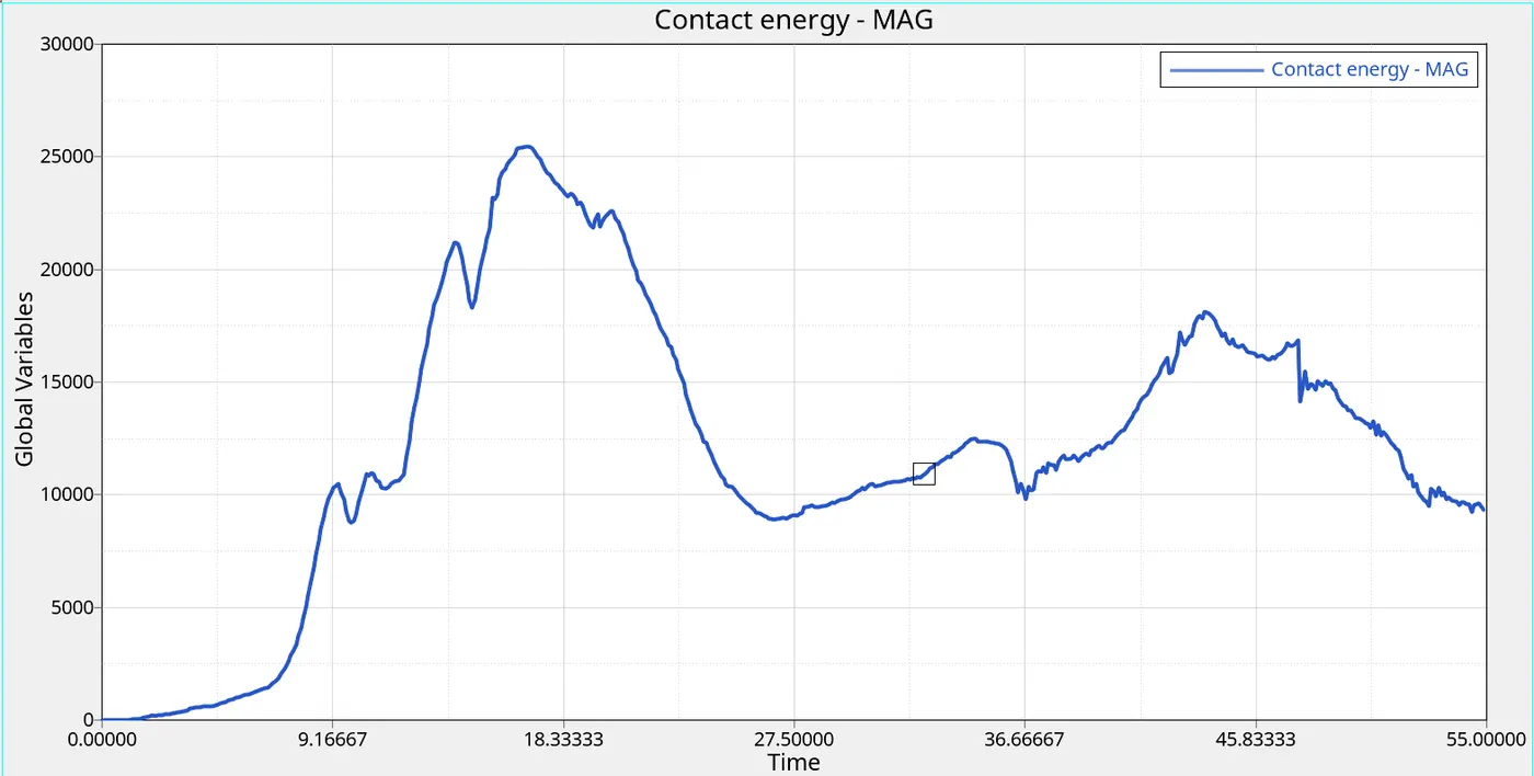
6. Contact Energy in Case 2 has much steeper graph compared to case 1, due to the second collision of the bend with the rigid wall.
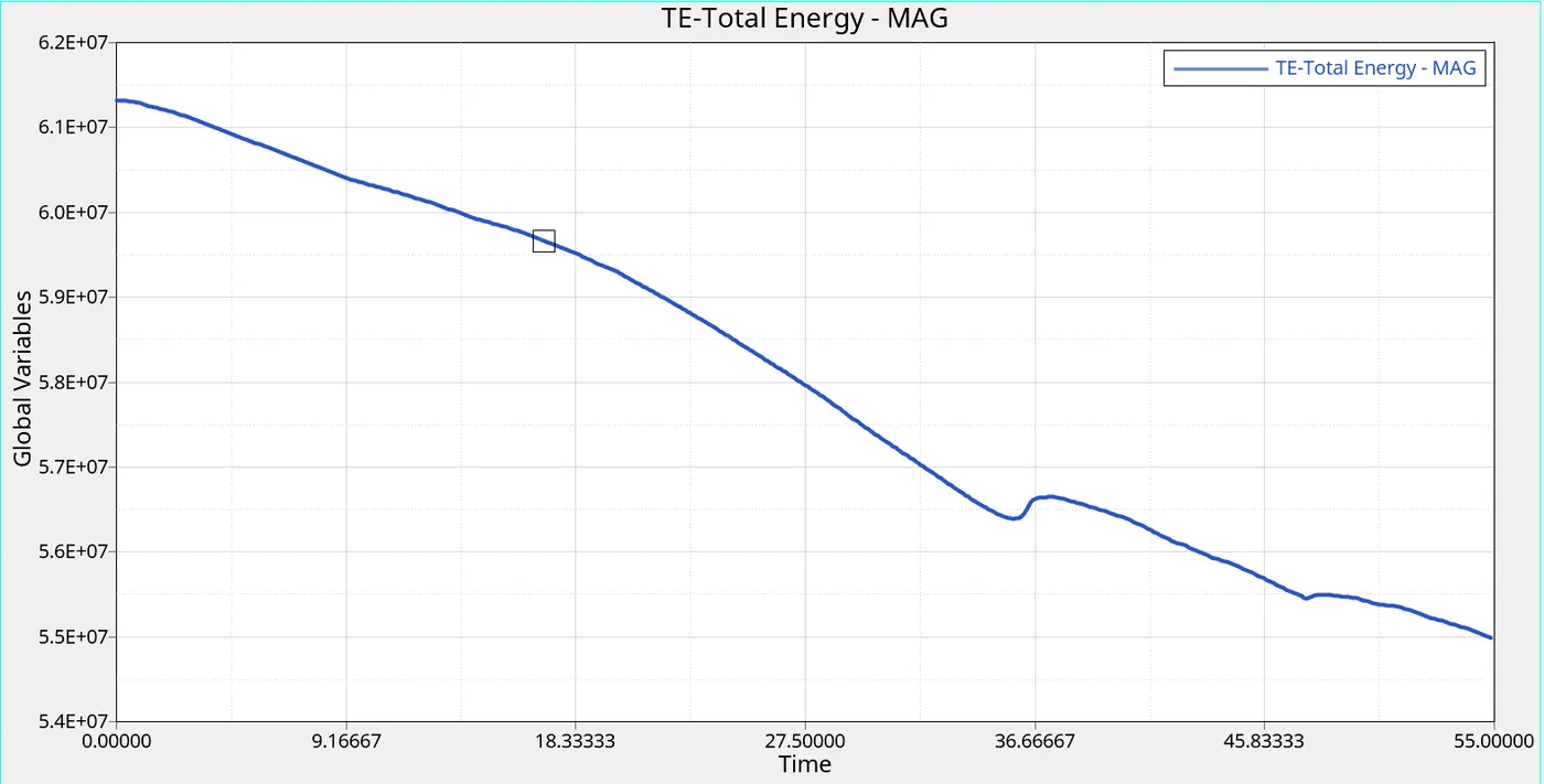
7. Total Energy in Case 1 decreases to 5.5E+07, while the same in Case 2 decreases to 6.126E+07. Thus, in Case 1, more energy loss occured compared to Case 2, at the end of the simulation. This is due to the loss of energy due to Hourglassing in Case 1.
8. Thus we can see that there is a large difference in the deformation behaviour and hourglass behaviour between the two cases, which leads to large variations in Total Energy at the end of the simulation.
This highlights the significance of choosing the property values correctly.
E. Conclusion
1. From above summary it is clear that choice of element formulation flag is one of the most important steps in an analysis.
2. In this case since the deformations are very large, the Case 1 choice of element formulation flag (default - 1) was wrong, which was giving rise to large amount of hourglassing energy.
In order to control hourglassing with large deformation, QEPH is a better choice of element formulation flag.
3. Case 2 was a better and more realistic simulation of the crash.
F. Hourglassing and how to control/minimise it:
1. In four noded shell elements, the property values are calculated over the element at the Gaussian integration points. These can be either 4 or 1. The more the number of integration points, the better is the accuracy of the simulation.
2. In 1 point integration elements, there can be 0 overall strain occuring at the integration point. This creates problems as the algorithm assumes the element has not deformed and hence no stress is registered. This leads to the element deforming unnaturally.
3. This kind of distortion introduces an energy loss called Hourglassing.
4. There are a few ways to control/minimise Hourglassing.
- Using 4 integration point elements: This method is computationally expensive but the most accurate. Using QBAT element type, we can get the best results at the cost of computational power.
- Using Hourglass stabilization - Perturbation method: In this case a damping factor is used to control unnatural deformation of the element. Element formulation flag: Ishell = 1,2,3, or 4
- Using Hourglass stabilization - Physical method : In this case the stiffness of the material is changed to achieve better hourglassing control. This method is more accurate than Perturbation method but increases the overall stiffness of the material. Element formulation flag: Ishell = 24