2D Element Formulation

OBJECTIVE: Aim of this challenge is to compare the results of simulation between the two cases in the same model. Case 1 simulation is done without assigning any property value while the case 2 simulations is run with all the recommended values.

PROBLEM STATEMENT:

• Using the crash beam file from the previous assignment, change the run time to 55ms.
• Change the number of animation steps during simulation to a minimum of 25 and a maximum of 60
• Run the base simulation without any modification to element properties.
• At the end of the simulation, do the energy error and mass error checks and determine whether the results would be acceptable.
• If acceptable, Plot rigid wall forces, internal energy, hourglass energy, contact energy, the total energy of the simulations.
• Change all the shell elements properties to recommended properties, save this as separate, rad files, and run the simulation.
• Follow steps 5 and 6.
• Create a brief report comparing all the results from steps 5 and 6 for both simulations.
• Comment whether there is any change in the results and why there is any change in the result.

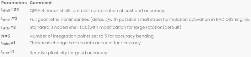
RECOMMENDED PROPERTIES:

PROCEDURE:

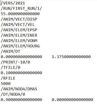
STEP-1: Edit the engine file. Open the engine file with notepad and edit the value of runtime from 60 to 55. Do not disturb the standard form of the number. Further, calculate the frequency of the animation for 40 animations. This can be calculated by dividing the number of animations by runtime. Thus f=55/40= 1.375. Change the end frequency value in the engine file and save the text file.

CASE-1

STEP-2: Import the solver deck and Run simulation. Go to Import< Solver deck and select 0000.rad file and hit import. Then go to Analysis< Radioss and put the option's value as –nt 4 for faster simulation and hit radioss to start the simulation process.

STEP-3: Open Hyperview to run the animation. Open the .hrd file that contains every animation file created during the simulation. Here we can check displacement, hourglass energy, von mises stress values, etc. Select the option accordingly and run the animation to see the component deform due to applied load.

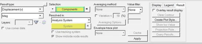
STEP-4: Open Hypergraph 2D to get the required graphs. Open T01 file that was created during the simulation process. Here we can plot the energy graphs and Rwall forces.

CASE-2

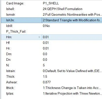
STEP-2: Import the solver deck, enter recommended property values and run the simulation. We can assign the values by going to the property, selecting them, and entering the values accordingly.

Note: The rest of the procedure remains the same as mentioned earlier.

GRAPH INFERENCE:

GRAPH-1: ENERGY CURVE

CASE-1:

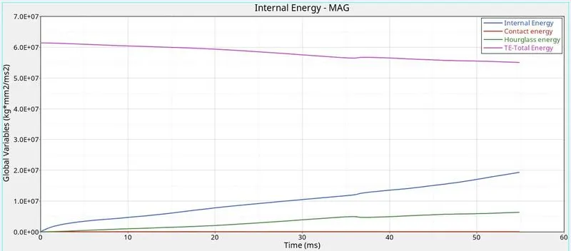
• The total energy is decreasing gradually which makes sense because the energy error for the first case ranges from 0% to -10%
• Internal energy is zero in the beginning and then gradually increases because there is was no strain initially and as the load has applied a strain is generated in the component due to deformation.
• Contact energy remains zero and constant throughout the simulation.
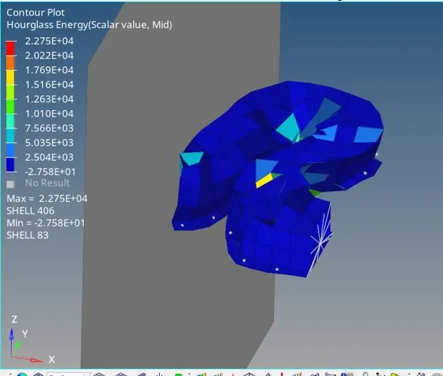
• Hourglass energy increases gradually which means that in case-1 there are a lot of elements that are deforming but still have zero stress.

CASE-2:

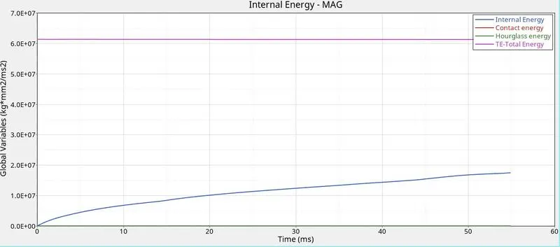
• The total energy in this case is almost constant. Even if it looks constant, there is still a -0.1% energy error in the output file.
• Internal energy is gradually increasing from zero in the beginning due to the same reason mentioned for case 1.
• Contact energy remains zero and constant throughout the simulation.
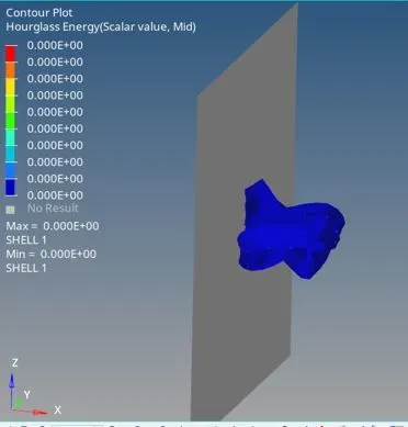
• Hourglass energy is also zero which signifies that there are no to little elements that have no stress.

GRAPH-2: RIGID WALL FORCES

CASE-1:

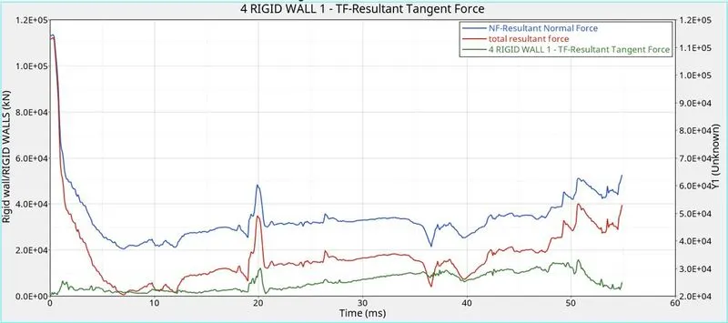
CASE-2:

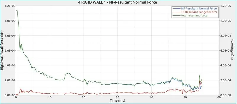
• Here the total resultant force is high initially because of the applied load at the rigid mass opposite to the rigid wall.
• The force comes down because the deformation starts in the model which gives rise to other forces that oppose the applied load.

GRAPH COMPARISON:

• The total energy curve gradually decreases in case-1 while in case-2 it is almost constant. This makes sense because there is a great difference between their energy error values.
• Internal energy curves in both cases gradually increase. However, the value of internal energy is more for case-2 at any point.
• There is a vast difference between the hourglass energies curves. In case-1 it is gradually increasing while in case-2 it is almost zero. Choosing QEPH element does give a better result.
• The resultant force in case-1 falls abruptly when compared to case-2. This implies that case-2 elements deform gradually and case-1 elements deform quickly (initially).

MORE COMPARISON BETWEEN BOTH THE CASES:

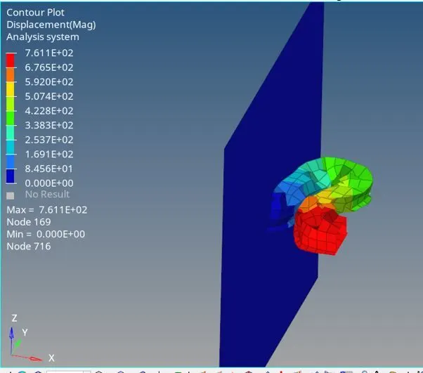
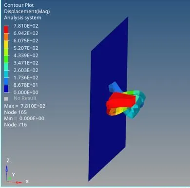
DISPLACEMENT:

CASE-1

CASE-2

HOURGLASS ENERGY:

CASE-1:

CASE-2

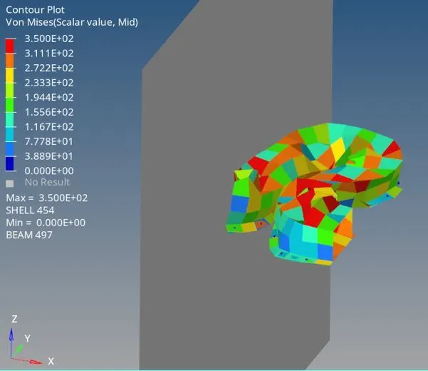
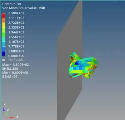
VON-MISSES STRESS:

CASE-1

CASE-2

REASONS FOR THE CHANGE:

As mentioned earlier, there is a humongous change in the results between both cases. The reason for this is pretty obvious. In case-1 we ran the simulation at default values, but in case-2 we assigned certain values in the property card before running the simulation. Given below is a brief comparison of how changing these values helped in getting a better result.

• Changing Ishell from default 1 to 24: Even if both the values contain 1 gauss point or integration point, QEPH elements that are Ishell=24 employees physical method to stabilize hourglassing. In this method, the stiffness is added to the element at the material level, changing its property, and the hourglass is taken care of even before arising. Whereas, in the Q4 element, the perturbation method is used in which the stiffness is added after the hourglass is detected, giving rise to a lot of hourglass energy.
• Changing N value from 0 to 5: This means that we are adding integration points throughout the thickness of the element. These integration points help with the accuracy.
• Changing Ithick value from 2 to 1: In the plastic region, the thickness of the component might not the constant like in the initial stages or in the elastic region. The default value of 2 does not account for this change while changing the value to 1 takes this change into account. Thus, we get better accuracy in calculation.
• Changing Iplas value from 2 to 1: In the plastic region, beyond the yield point, the default value of 2 does not update strain through the thickness and calculates new values according to the changing thickness due to deformation. While, by changing the value to 1, we might take some extra time to calculate the values, the solver takes the mentioned steps into account and provide accurate results.
• We did not change the values of Ismstr and Ish3N because the default value is also 2.

CONCLUSION: Through this assignment, I have learned to run simulations, read engine output files, plot graphs, run animations, and compare the graphs of the same model under different property values.