Otto cycle

Objective: Program for obtaining volume v/s pressure plot of Otto cycle and output the thermal efficiency.

Otto cycle:

The Otto cycle describes how heat engines turn gasoline into motion. Like other thermodynamic cycles, this cycle turns chemical energy into thermal energy and then into motion.

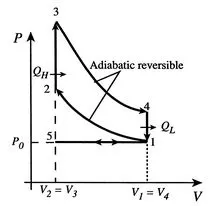
Figure: Ideal otto cycle

The ideal Otto cycle consists of four internal reversible processes:

1-2 Isentropic compression.

2-3 Constant volume, heat addition.

3-4 Isentropic expansion.

4-1 Constant volume, heat rejection.

Input parameters: Swept volume (v1), t1, t3, Compression ratio (Cr).

Engine Geometric parameters:

• Bore.
• Stroke.
• Connecting rod length.
• Compression Ratio- The compression ratio (Cr) is the ratio of total cylinder volume to the clearance volume.
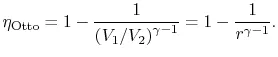
  Thermal efficiency:

MATLAB Program to plot the Otto cycle:

clear all
close all
clc

%Input
gamma=1.4;

%state variable
p1=101325;
t1=500;
t3=500;

%engine geometric parameters 
bore=0.1;
stroke=0.1;
conn_rod=0.15;
Cr=12;

%Calculating swept volume and clearance volume
v_swept=(pi/4)*bore^2*stroke;
v_clearance=v_swept/(Cr-1);

v1=v_swept+v_clearance;
v2=v_clearance;

%Compression curve
V_compression=Piston_kinematics(bore,stroke,conn_rod,Cr,0,180);
constant1=p1*v1^gamma;
P_compression= constant1./V_compression.^gamma;

%state variables at state 2
%p2v2^gamma=p1v1^gamma
%Cr=v1/v2
p2=p1*Cr^gamma;

%p1v1/t1=p2v2/t2
t2=p2*v2*t1/(p1*v1);

%state variable at state 3
v3=v2;
%p3v3/t3=p2v2/t2
p3=p2*t3/t2;

%Expansion curve
V_expansion=Piston_kinematics(bore,stroke,conn_rod,Cr,0,180);
constant2=p3*v3^gamma;
P_expansion= constant2./V_compression.^gamma;

%state variable at state 4
v4=v1;

%p3v3^gamma=p4v4^gamma
p4=p3*(v3/v4)^gamma;

figure(1)
hold on
plot(v1,p1,'*','color','b')
plot(V_compression,P_compression,'color','r')
plot(v2,p2,'*','color','b')
plot([v2 v3],[p2 p3],'color','g')
plot(v3,p3,'*','color','b')
plot(V_expansion,P_expansion,'color','r')
plot([v4 v1],[p4 p1],'color','g')
plot(v4,p4,'*','color','b')
xlabel('Volume')
ylabel('Pressure')

%thermal efficiency of otto cycle
thermal_efficiency=(1-(1/Cr^(gamma-1)))*100

Explanation of the program:

1. At first, provide the input parameters which are p1, t1, t3, and gamma then put in the engine geometric parameters.
2. Then calculate the swept volume and clearance volume by using the respective formula and further calculate the total volume (v1) and define (v2).
3. In the next step, call in the engine_kinematics function that we have already defined in order to find the v_compression value and further calculate p_compression, this step is going to give the curve for isentropic compression of Otto cycle.
4. Similarly, define the state variables of state 2, and 3 and call in the function engine_kinematics to find out the v_expansion and p_expansion for the isentropic expansion curve of the Otto cycle.
5. Further, input the variables of state 4 and plot all of the state variables shown by ‘*’ in the figure(1).
6. Then plot a straight line, connecting state variable 2 to 3(constant volume heat addition), and 4 to 1(constant volume heat rejection).
7. And further, also plot the compression and expansion curve by connecting the state variable 1 to 2(isentropic compression) and 3 to 4(isentropic expansion) and label the x-axis and y-axis.
8. Lastly, put the formula of thermal efficiency in order to get the output which is dependent on the gamma and the compression ratio.

The figure shows the plot of Volume vs pressure of the Otto cycle:

The workspace of Matlab is on the left and the command window to the right shows the output as thermal efficiency of the Otto cycle:

Output: The thermal efficiency of the otto cycle is 62.989%.

References:

https://energyeducation.ca/encyclopedia/Otto_cycle

http://mechteacher.com/otto-cycle-air-standard-efficiency-derivation/#ixzz6UECTvQI7