Analysis of Popular Baby Names Database using Python Libraries
Here, an effort is made to determine the common baby names as Word Cloud among various ethnicities, years, and gender using Python in Jupyter Notebook. An arbitrary file available on the internet is downloaded and processed.
The same .csv file can be obtained from the following link: <https://drive.google.com/drive/folders/1SpQr865ckvhPsrulHRJ7mZ9TfH1yKJf3?usp=sharing>
Before we begin with, we check how the data is mentioned in the file.
import pandas as pd
names_data = pd.read_csv('baby_names.csv')
names_data.info()
names_data.head()
Output:
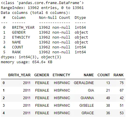
Now, let us check the count of values in each column.
names_data["BRITH_YEAR"].value_counts()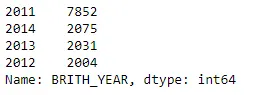
names_data["GENDER"].value_counts()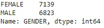
names_data["ETHNICTY"].value_counts()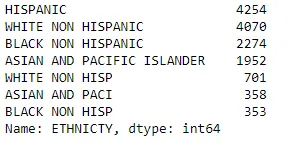
As can be observed from the above output, there are multiple entries for the same ethnicity for eg., "WHITE NON HISPANIC" and "WHITE NON HISP". So they are replaced by the same value.
#Cleaning the data by replacing the shortcuts for ethnicty
names_data["ETHNICTY"]=names_data["ETHNICTY"].str.replace("WHITE NON HISPANIC","WHITE NON HISP")
names_data["ETHNICTY"]=names_data["ETHNICTY"].str.replace("BLACK NON HISPANIC","BLACK NON HISP")
names_data["ETHNICTY"]=names_data["ETHNICTY"].str.replace("ASIAN AND PACIFIC ISLANDER","ASIAN AND PACI")
names_data["ETHNICTY"].value_counts()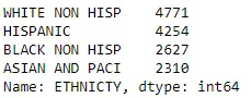
Now, let us come to the "NAME" column, where all the strings are converted to either "Upper Case" or "Lower Case" to identify the duplicate entries, removing unwanted columns, and finalize the entries.
# using the upper case for all the names # to overcome if any names entered in lowercase
names_data["NAME"]=names_data["NAME"].str.upper()
#removing the duplicate entry
names_data.drop_duplicates(keep='first',inplace=True)
names_data=names_data.drop(['RANK'], axis=1)
names_data.info()
# this is the final refined list of the data
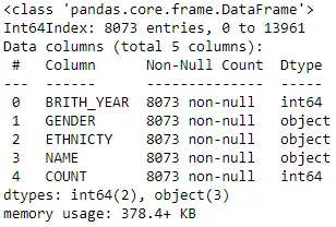
Once the duplicate entries are removed, the data is refined to 8073 entries from 13962 entries. This is the final list we will be working on.
GenderWise Data:
Let us see how the data is segregated in terms of gender.
#Gender wise size
import matplotlib.pyplot as plt
names_data5=names_data
names_data5=names_data5.groupby(['GENDER']).COUNT.sum().to_frame(name='COUNT').reset_index().sort_values('COUNT', ascending =False)
names_data5['percentage']=(names_data5['COUNT']/names_data5['COUNT'].sum(axis=0))*100

explode = (0, 0.1)
fig1, ax1 = plt.subplots()
ax1.pie(names_data5['percentage'], explode=explode, labels=names_data5['GENDER'], autopct='%1.1f%%',
        shadow=True, startangle=90)
ax1.axis('equal')  # Equal aspect ratio ensures that pie is drawn as a circle.

plt.show()
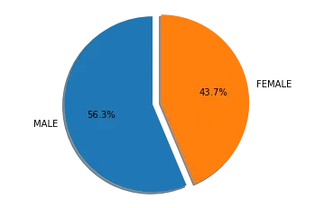
Out of all the entries, 56.3% are MALE and 43.7% are FEMALE.
Ethnicity Wise Data:
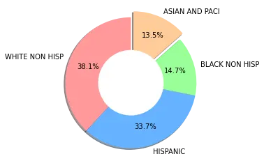
Let us see how the data is segregated in terms of ethnicity.
#Ethnicty wise sample size
names_data6=names_data
names_data6=names_data6.groupby(['ETHNICTY']).COUNT.sum().to_frame(name='COUNT').reset_index().sort_values('COUNT', ascending =False)

names_data6['percentage']=(names_data6['COUNT']/names_data6['COUNT'].sum(axis=0))*100

explode = (0, 0,0,0.1)
colors = ['#ff9999','#66b3ff','#99ff99','#ffcc99']
fig1, ax1 = plt.subplots()
ax1.pie(names_data6['percentage'], explode=explode, labels=names_data6['ETHNICTY'], autopct='%1.1f%%',
        shadow=True, startangle=90, pctdistance = 0.7, colors = colors)
ax1.axis('equal')  # Equal aspect ratio ensures that pie is drawn as a circle.
#draw circle
centre_circle = plt.Circle((0,0),0.5,fc='white')
fig = plt.gcf()
fig.gca().add_artist(centre_circle)

plt.show()
names_data7=names_data
names_data7=names_data7.groupby(['ETHNICTY','GENDER']).COUNT.sum().to_frame(name='COUNT').reset_index()
names_data7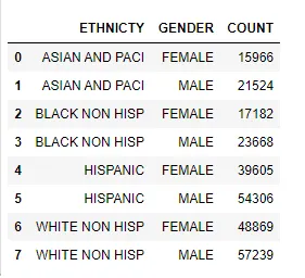
Now calculating the percentage of males and females for each ethnic group.
#names_data8=pd.DataFrame(columns=['ETHNICTY','MALE','FEMALE'])

names_data8=names_data7.pivot(index ='ETHNICTY', columns='GENDER', values ='COUNT').reset_index().rename_axis(None)
names_data8['Total']=names_data8['FEMALE']+names_data8['MALE']
names_data8['Female_percent']=(names_data8['FEMALE']/names_data8['FEMALE'].sum(axis=0))*100
names_data8['Male_percent']=(names_data8['MALE']/names_data8['MALE'].sum(axis=0))*100
names_data8['Total_percent']=(names_data8['Total']/names_data8['Total'].sum(axis=0))*100
names_data8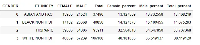
import matplotlib.patches as mpatches
colors = ['#ff9999','#66b3ff','#99ff99','#ffcc99']

colors_gender = ['#c2c2f0','#ffb3e6', '#c2c2f0','#ffb3e6', '#c2c2f0','#ffb3e6', '#c2c2f0','#ffb3e6']


explode = (0.3,0.3,0.3,0.3)
explode_gender = (0.3,0.3,0.3,0.3,0.3,0.3,0.3,0.3)

fig1, ax1 = plt.subplots(figsize=(10, 10))
ax1.pie(names_data8['Total_percent'], labels=names_data8['ETHNICTY'], autopct='%1.1f%%',
        shadow=True, startangle=90, pctdistance = 0.8,explode = explode, colors = colors,radius=8)
#fig1,ax2 =plt.subplots()
ax1.pie(names_data7['COUNT'],
        shadow=True, autopct='%1.1f%%',startangle=90, pctdistance = 0.7, colors=colors_gender,radius=5,explode = explode_gender)

ax1.axis('equal')  # Equal aspect ratio ensures that pie is drawn as a circle.
#draw circle
centre_circle = plt.Circle((0,0),3,fc='white')

fig = plt.gcf()
fig.gca().add_artist(centre_circle)


gend=["MALE","FEMALE"]


from matplotlib.lines import Line2D
custom_lines = [Line2D([0], [0], color='#ffb3e6', lw=6),
                Line2D([0], [0], color='#c2c2f0', lw=6)]

ax1.legend(custom_lines, gend,loc="center").get_frame().set_linewidth(0.0)
#<.get_frame().set_edgecolor('b')> to set the border color of legend


plt.show()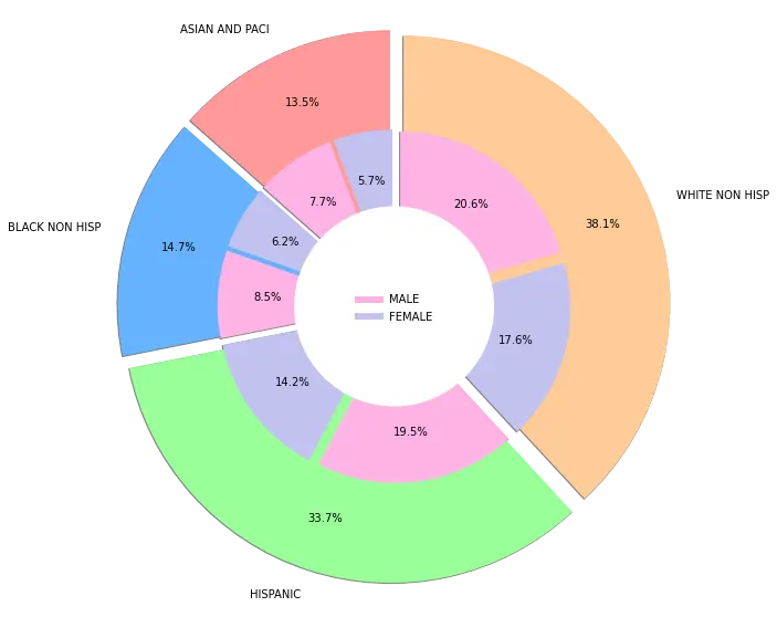
Analysis:
Grouping Data by Name and Gender:
Here the data is grouped by Name and Gender for all the years and in the count column all the cumulative sums are stored and a new frequency column is added to determine the repeating frequency of the names.
# to find most common names of all years 2011-14 for both male and female
names_data1=names_data
names_data1=names_data1.drop(['ETHNICTY'], axis=1)
names_data1=names_data1.groupby(['GENDER','NAME']).COUNT.sum().to_frame(name='COUNT').reset_index()
names_data1.sort_values('COUNT', ascending =False)
names_data1_male = names_data1[names_data1['GENDER']=='MALE'].sort_values('COUNT', ascending =False)
names_data1_female = names_data1[names_data1['GENDER']=='FEMALE'].sort_values('COUNT', ascending =False)
names_data1_male['frequency']=(names_data1_male['COUNT']/names_data1_male['COUNT'].sum(axis=0))*100
names_data1_female['frequency']=(names_data1_female['COUNT']/names_data1_female['COUNT'].sum(axis=0))*100
Now a word cloud is formed using the Names and frequency for each gender.
Most Common Name of Male Children for all the years:
#most common name among male children for all years
d= dict(zip(names_data1_male['NAME'],names_data1_male['frequency']))

import matplotlib.pyplot as plt
from wordcloud import WordCloud

wordcloud = WordCloud(background_color="white")
wordcloud.generate_from_frequencies(frequencies=d)
plt.figure()
plt.imshow(wordcloud, interpolation="bilinear")
plt.axis("off")
plt.show()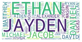
Most Common Name of Female Children for all the years:
#most common name among female children for all years
d= dict(zip(names_data1_female['NAME'],names_data1_female['frequency']))

import matplotlib.pyplot as plt
from wordcloud import WordCloud

wordcloud = WordCloud(background_color="white")
wordcloud.generate_from_frequencies(frequencies=d)
plt.figure()
plt.imshow(wordcloud, interpolation="bilinear")
plt.axis("off")
plt.show()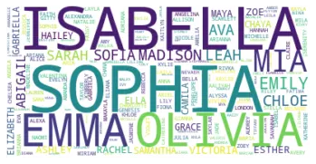
Now the data is segregated in terms of ethnicity and the frequency of each name among males and females column are added as shown below.
names_data2=names_data

names_data2=names_data2.set_index(['GENDER','ETHNICTY','NAME','BRITH_YEAR']).sort_index(level=0)
names_data2=names_data2.groupby(['GENDER','ETHNICTY','NAME']).COUNT.sum().to_frame(name='COUNT').reset_index()


names_data2_AnP = names_data2[names_data2['ETHNICTY']=='ASIAN AND PACI'].sort_values('COUNT', ascending =False)
names_data2_AnP['frequency']=(names_data2_AnP['COUNT']/names_data2_AnP['COUNT'].sum(axis=0))*100

names_data2_Hisp = names_data2[names_data2['ETHNICTY']=='HISPANIC'].sort_values('COUNT', ascending =False)
names_data2_Hisp['frequency']=(names_data2_Hisp['COUNT']/names_data2_Hisp['COUNT'].sum(axis=0))*100

names_data2_BnH = names_data2[names_data2['ETHNICTY']=='BLACK NON HISP'].sort_values('COUNT', ascending =False)
names_data2_BnH['frequency']=(names_data2_BnH['COUNT']/names_data2_BnH['COUNT'].sum(axis=0))*100

names_data2_WnH = names_data2[names_data2['ETHNICTY']=='WHITE NON HISP'].sort_values('COUNT', ascending =False)
names_data2_WnH['frequency']=(names_data2_WnH['COUNT']/names_data2_WnH['COUNT'].sum(axis=0))*100

names_data2_AnP_male=names_data2_AnP[names_data2_AnP['GENDER']=='MALE'].sort_values('COUNT', ascending =False)
names_data2_AnP_male['frequency']=(names_data2_AnP_male['COUNT']/names_data2_AnP_male['COUNT'].sum(axis=0))*100

names_data2_AnP_female=names_data2_AnP[names_data2_AnP['GENDER']=='FEMALE'].sort_values('COUNT', ascending =False)
names_data2_AnP_female['frequency']=(names_data2_AnP_female['COUNT']/names_data2_AnP_female['COUNT'].sum(axis=0))*100

names_data2_Hisp_male=names_data2_Hisp[names_data2_Hisp['GENDER']=='MALE'].sort_values('COUNT', ascending =False)
names_data2_Hisp_male['frequency']=(names_data2_Hisp_male['COUNT']/names_data2_Hisp_male['COUNT'].sum(axis=0))*100

names_data2_Hisp_female=names_data2_Hisp[names_data2_Hisp['GENDER']=='FEMALE'].sort_values('COUNT', ascending =False)
names_data2_Hisp_female['frequency']=(names_data2_Hisp_female['COUNT']/names_data2_Hisp_female['COUNT'].sum(axis=0))*100

names_data2_BnH_male=names_data2_BnH[names_data2_BnH['GENDER']=='MALE'].sort_values('COUNT', ascending =False)
names_data2_BnH_male['frequency']=(names_data2_BnH_male['COUNT']/names_data2_BnH_male['COUNT'].sum(axis=0))*100

names_data2_BnH_female=names_data2_BnH[names_data2_BnH['GENDER']=='FEMALE'].sort_values('COUNT', ascending =False)
names_data2_BnH_female['frequency']=(names_data2_BnH_female['COUNT']/names_data2_BnH_female['COUNT'].sum(axis=0))*100

names_data2_WnH_male=names_data2_WnH[names_data2_WnH['GENDER']=='MALE'].sort_values('COUNT', ascending =False)
names_data2_WnH_male['frequency']=(names_data2_WnH_male['COUNT']/names_data2_WnH_male['COUNT'].sum(axis=0))*100

names_data2_WnH_female=names_data2_WnH[names_data2_WnH['GENDER']=='FEMALE'].sort_values('COUNT', ascending =False)
names_data2_WnH_female['frequency']=(names_data2_WnH_female['COUNT']/names_data2_WnH_female['COUNT'].sum(axis=0))*100
Most common name among all children (Asia Pacific) for all years:
#most common name among all children (Asia Pacific) for all years
d= dict(zip(names_data2_AnP['NAME'],names_data2_AnP['frequency']))

import matplotlib.pyplot as plt
from wordcloud import WordCloud

wordcloud = WordCloud(background_color="white")
wordcloud.generate_from_frequencies(frequencies=d)
plt.figure()
plt.imshow(wordcloud, interpolation="bilinear")
plt.axis("off")
plt.show()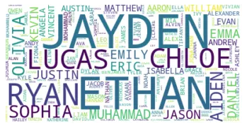
Most common name among all children (Hispanic) for all years:
#most common name among all children (Hispanic) for all years
d= dict(zip(names_data2_Hisp['NAME'],names_data2_Hisp['frequency']))

import matplotlib.pyplot as plt
from wordcloud import WordCloud

wordcloud = WordCloud(background_color="white")
wordcloud.generate_from_frequencies(frequencies=d)
plt.figure()
plt.imshow(wordcloud, interpolation="bilinear")
plt.axis("off")
plt.show()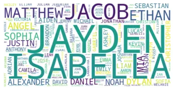
Most common name among all children (Black Non Hispanic) for all years:
#most common name among all children (Black non Hispanic) for all years
d= dict(zip(names_data2_BnH['NAME'],names_data2_BnH['frequency']))

import matplotlib.pyplot as plt
from wordcloud import WordCloud

wordcloud = WordCloud(background_color="white")
wordcloud.generate_from_frequencies(frequencies=d)
plt.figure()
plt.imshow(wordcloud, interpolation="bilinear")
plt.axis("off")
plt.show()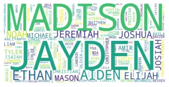
Most common name among all children (White Non Hispanic) for all years:
#most common name among all children (White non Hispanic) for all years
d= dict(zip(names_data2_WnH['NAME'],names_data2_WnH['frequency']))

import matplotlib.pyplot as plt
from wordcloud import WordCloud

wordcloud = WordCloud(background_color="white")
wordcloud.generate_from_frequencies(frequencies=d)
plt.figure()
plt.imshow(wordcloud, interpolation="bilinear")
plt.axis("off")
plt.show()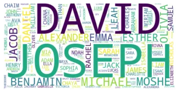
Most common name among Males (Asia Pacific) for all years:
#most common name among all male child (Asia Pacific) for all years
d= dict(zip(names_data2_AnP_male['NAME'],names_data2_AnP_male['frequency']))

import matplotlib.pyplot as plt
from wordcloud import WordCloud

wordcloud = WordCloud(background_color="white")
wordcloud.generate_from_frequencies(frequencies=d)
plt.figure()
plt.imshow(wordcloud, interpolation="bilinear")
plt.axis("off")
plt.show()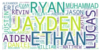
Most common name among Females (Hispanic) for all years:
#most common name among all female child (Hispanic) for all years
d= dict(zip(names_data2_Hisp_female['NAME'],names_data2_Hisp_female['frequency']))

import matplotlib.pyplot as plt
from wordcloud import WordCloud

wordcloud = WordCloud(background_color="white")
wordcloud.generate_from_frequencies(frequencies=d)
plt.figure()
plt.imshow(wordcloud, interpolation="bilinear")
plt.axis("off")
plt.show()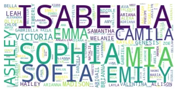
Most Popular Name in 2011:
#2011 popular male name
names_data3=names_data

#names_data3.set_index(['BRITH_YEAR','GENDER','NAME']).sort_index(level=0)
#names_data3.groupby(['GENDER','NAME']).COUNT.sum().to_frame(name='COUNT').reset_index()

names_data3=names_data3[names_data3['BRITH_YEAR']==2011].sort_values('COUNT', ascending =False)
names_data3=names_data3[names_data3['GENDER']=="MALE"]
names_data3=names_data3.drop(['ETHNICTY'], axis=1)
names_data3=names_data3.groupby(['NAME']).COUNT.sum().to_frame(name='COUNT').reset_index().sort_values('COUNT', ascending =False)

names_data3['frequency']=(names_data3['COUNT']/names_data3['COUNT'].sum(axis=0))*100

d= dict(zip(names_data3['NAME'],names_data3['frequency']))

import matplotlib.pyplot as plt
from wordcloud import WordCloud

wordcloud = WordCloud(background_color="white")
wordcloud.generate_from_frequencies(frequencies=d)
plt.figure()
plt.imshow(wordcloud, interpolation="bilinear")
plt.axis("off")
plt.show()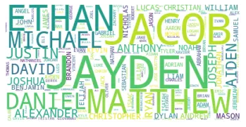
Most Popular Female Name among Hispanic in the year 2014:
#2014 popular female name among Hispanic
names_data4=names_data

names_data4=names_data4[names_data4['BRITH_YEAR']==2014].sort_values('COUNT', ascending =False)
names_data4=names_data4[names_data4['GENDER']=="FEMALE"].sort_values('COUNT', ascending =False)
names_data4=names_data4[names_data4['ETHNICTY']=="HISPANIC"].sort_values('COUNT', ascending =False)

names_data4=names_data4.drop(['ETHNICTY','GENDER','BRITH_YEAR'], axis=1)
names_data4.groupby(['NAME']).COUNT.sum().to_frame(name='COUNT').reset_index().sort_values('COUNT', ascending =False)

names_data4['frequency']=(names_data4['COUNT']/names_data4['COUNT'].sum(axis=0))*100

d= dict(zip(names_data4['NAME'],names_data4['frequency']))

import matplotlib.pyplot as plt
from wordcloud import WordCloud

wordcloud = WordCloud(background_color="white")
wordcloud.generate_from_frequencies(frequencies=d)
plt.figure()
plt.imshow(wordcloud, interpolation="bilinear")
plt.axis("off")
plt.show()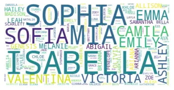
Conclusions:
- Various commands of data interpretation are used viz., value_counts(), str.replace(). str.upper(), drop_duplicates(), drop(), info(), word cloud plotting, COUNT, sum, sort_values() etc.,
<code and data file can be found in the link above>